Descripción
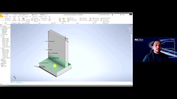
Real-world problems are rarely linear or static. Nonlinearities often impact the prediction of a product's behavior in unpredictable ways. These add uncertainty and risk to decisions made from either virtual or physical test results for engineers and designers who don't understand them. In this presentation we’ll use Inventor Nastran software to mid-surface a thin-walled assembly and weld the parts together. We’ll then go through the process of validating our model and then performing a nonlinear static analysis with linear and then nonlinear materials. Once the existing design is validated, we’ll perform a light-weighting design optimization to reduce the assembly’s weight, and then we’ll perform a nonlinear verification analysis on the final, reduced-weight design.
Aprendizajes clave
- Learn how to mid-surface and mesh solid geometry to generate a shell mesh.
- Learn how to connect shell meshed parts in an assembly using offset welded contact.
- Learn how to define nonlinear materials and large displacement effects, and perform a nonlinear analysis.
- Learn how to lightweight an existing shell meshed design using Autodesk Nastran SIMP Topology Optimization.
Downloads
Etiquetas
Producto | |
Sectores | |
Temas |
A la gente que le gusta esta clase también gusta
Instructional Demo
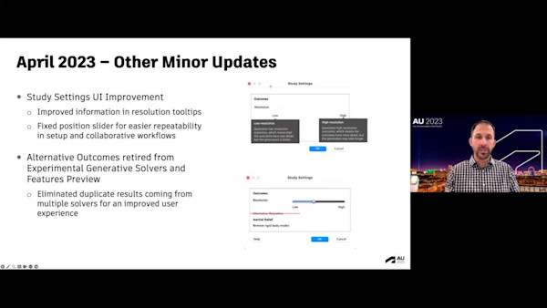
Success with Generative Design in 2023


Instructional Demo
Automated Bridge Design Workflow: The Road to Detailed Design
Instructional Demo