Summary
- This blog post goes through the InfoWorks ICM troubleshooting procedure we use when helping customers and includes common things to look out for.
- It is not exhaustive and focuses on simulation convergence rather than initialization.
- Many of the issues reported above could also lead to initialization failures. In most cases, a better schematized and convergent model should run faster.
We often get asked about troubleshooting models. Here is the best advice we’ve collected from speaking to customers in-depth – here’s what we recommend you do when you need to understand what went wrong.
To begin with, troubleshooting a problematic, non-convergent model can be avoided by following best practices, providing sensible and well thought schematization, and paying close attention to validation errors and warnings.
The first things we do
We find it useful to build models iteratively, testing the model out at various stages. For instance, test it as a 1D river model before merging with a 1D urban drainage model, before merging with a simple 2D mesh, before adding mesh detail, etc. It may feel more time-consuming in the short term, but in our experience it helps solves many issues and actually speeds up the entire modeling process.
Whenever we get sent an integrated 1D-2D model, the first thing we do is turn off 2D details by setting bank discharge coefficients to 0 and all 2D nodes to sealed flood types. That way, you can check to see how the 1D model works on its own.
Checking the simulation log files
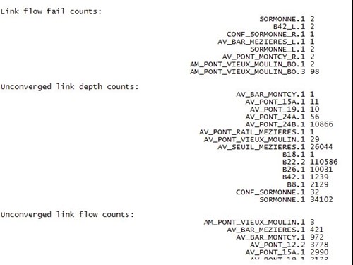
The first glimmer of a notice of when a model is non-convergent will be the premature failure of the simulation. You’ll see the simulation icon in the database tree turn red. We always advise reviewing log files regardless of the simulation status. You should begin by taking a look at the simulation log file (right click on the simulation icon; ‘Open As…Log Results’). Scroll down to the bottom of the log file. The final details will show where the convergence failure occurred and the point the simulation ultimately failed.

In most situations, it will be the locations noted in the screenshot above that are responsible for the simulation failure. Occasionally, the point of the final convergence failure is not always the real cause of the simulation failure.

Need more information to troubleshoot? In the run dialogue, under diagnostics, is the option to turn on the ‘Timestep log’. Switch this on for an enhanced and more comprehensive simulation log file, which provides convergence information for every timestep. Towards the point of the simulation failure, there will most likely be a particular location which regularly appears within the convergence failure information. Note that we recommend only using this option for troubleshooting as it results in very large log files.

Towards the bottom of the simulation log file, you will see a hit count of the link/node fail counts.

It is worth investigating the locations with the larger hit counts. For 1D-2D models, we advise checking the volume balance error in the 2D summary log. This should be close to 0%, although less than 5% is usually considered acceptable.

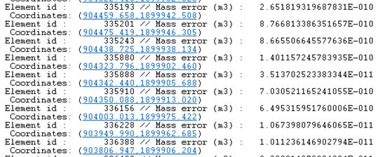
Where the volume balance error is greater than 5%, you’ll see a list of locations with their associated mass error. In nearly all cases these are associated with the 1D-2D interface. They may also be accompanied by messages about river bank flow oscillations. This is when flow oscillates from positive (flow from the river reach to the 2D zone) to negative (flow from the 2D zone back to the river reach). Of course, such oscillations can be natural, particularly when the count is small. However, where oscillations occur during nearly every results timestep, it may be indicative of an instability propagating across the 1D-2D interface.


Identifying poor convergence using the Results Grid
With the results open in the geoplan, it’s possible to check the volume balance on a node basis using the New Nodes Results Grid. These can be sorted to find the largest volume balance errors.

Finally, look for any oscillations in results where flow modes may be rapidly changing.
Once the poor convergence has been identified, at this stage you might be tempted to fiddle with your simulation parameters to force convergence, but we wouldn’t recommend this as quite often this will mask the issue and lead to other issues further down the line with different boundary conditions. We advise opening the results in the geoplan, finding the location specified in the simulation log file, and investigating both the model geometry and the results.
There are a number of typical reasons for simulation failures both within the 1D (both fluvial and urban drainage models) and 2D domains, which we’ll explore below.
Courant-Friedrich-Lewy Condition: How to choose your timestep size
In the large majority of cases, ensuring a timestep of 60 seconds or less and 10 seconds or less for 1D-2D simulations is recommended. The run timestep you specify in the schedule simulation dialog is the 1D timestep. The 2D timestep is determined by the Courant-Friedrich-Lewy Condition.
By default, the 1D and 2D engines will pass data at the run timestep provided in the schedule simulation dialog (known as the major timestep). However, when the 1D engine fails to converge, it will halve the timestep and try to iterate to converge towards a solution. The timestep used is called the minor timestep. Still, by default, the 1D and 2D engines pass data at the major timestep.
By ticking the option to ‘Link 1D and 2D Calculations at Minor Timestep’, where the 1D engine has timestep halvings, the 1D and 2D engines will pass data at this minor timestep. The option to ‘Link 1D and 2D Calculations at Minor Timesteps’ will ensure more interactions between the 1D and 2D models which can increase stability and reduce the volume balance error. Note that while this option can increase stability of models, it is not ticked by default because it can slightly increase run times.
Schematization issues
it would be impossible to go through the large number of potential reasons for poor convergence, but let’s talk about typical, common examples, along with some good approaches to addressing them.
Is it an initialization failure?
The first common issue often manifests itself as an initialization failure rather than a simulation failure, but it is worth pointing out here as it’s a regular issue in our support in-box that is easily spotted. It happens because of poor schematization, often where engineers have sampled bank-line elevations from a ground model but are picking up the channel as represented in the ground model rather than the banks.
Here is an example where the banklines are lower than the bed level of the river (thalweg). Often banklines can be low, but clearly this is very poor schematization.

In this situation, the only resolution is to improve the model schematization so that it better matches reality.
Check your steps in the river reach long profile
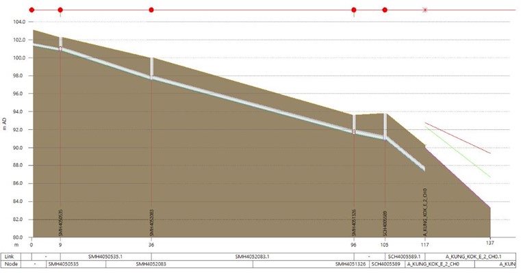
The next common issue involves large steps in the river reach long profile. These can often occur at structures or confluences due to poor schematisation or conflicting survey data. If the step occurs in reality, then any steps in the river reach profile typically greater than 1 in 10 should be represented as an irregular weir (or 1D inline bank). If the step does not exist in reality, then smoothing the transition should be considered.

This can also manifest itself in slightly different ways, such as soffit levels lower than downstream/upstream invert levels.

Related to this are outfalls from an urban drainage system into a river network with steep drops or poor schematisation. Occasionally, due to differences in surveyed data, we’ve seen model networks with outfalls entering the river either below the bed level or out of the bank. The outfalls should connect to a break node within the river and the connecting conduit should have a downstream invert level between the river section invert level and the bankline (in channel). The headloss type at the end of a sewer conduit connecting into a river should be set to either NONE or FIXED. NORMAL/HIGH headloss types are only appropriate at link ends connected to manholes.
A common issue with steep pipes
One common issue in pipe networks is seemingly random simulation failures, often in locations where steep conduits are present. As a very general rule, removing headlosses for conduits (usually at the upstream end) with a gradient greater than 0.1 (10%) can help with convergence.
Lack of panel markers and conflicting panel markers
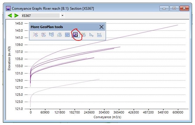
Occasionally, a lack of panel markers can lead to poor convergence within the simulation. Also common are conflicting panel markers for adjacent identical river sections (eg, two river reaches connected at a break node or a bridge section and the adjacent river reach section), which leads to very rapid changes in the conveyance profiles. These would need improved representation. You can use the tool “Conveyance graph pick” to plot several conveyance curves in the graph to do a direct comparison of adjacent curves.

Check your culvert inlets/outlets
The invert elevation at the end of a culvert conduit connected to a culvert inlet/outlet should be at the same level as the culvert inlet/outlet. Similarly, the lowest invert on a reach connected to a culvert inlet/outlet should also have the same invert level as the culvert inlet/outlet.
The headloss type at the end of the culvert conduit connected to the culvert inlet/outlet should be set to NONE. This is because the inlet/outlet is meant to incorporate all the losses between the reach and the culvert. The only exception to this is if bend losses are to be included, in which case a FIXED headloss with an appropriate coefficient should be used. NORMAL or HIGH headloss types should not be used in this situation.
Representing 1D structures in 2D
Quite often, you may have a requirement to represent structures within the 2D domain; for example, an opening in a railway embankment or underpass. Quite often, these are represented using 1D conduits coupled to the 2D using 2D outfalls. These can be tricky to set up in a stable manner, and we recommend that the conduit invert level matches the 2D outfall ground level and the mesh element elevation at each of the ends of the conduit. The 2D Outfall level ground level can be inferred from the 2D mesh using the inference tool, if required.
Ticking the option to ‘Link 1D and 2D Calculations at Minor Timesteps’ can also assist with the stability of these. Where a 2D outfall is used, the mesh element within which it resides should be large enough to contain the volume of flow which can enter the conduit. Alternatively, an inline bank could be used to represent a linear connection with multiple mesh elements. It is also possible to represent such structures in the 2d model directly using Base Linear Structures and Sluice/Bridge Linear Structures.
2D initial conditions…or lack thereof
The 2D engine itself is very stable. Most instabilities and poor convergence is associated with the 1D-2D interface. However, there have been instanced where users have applied a tidal level without the initial water level specified in the 2D domain, essentially applying a wall of water to the 2D domain.
Issues with modeling river banks
River reach banklines are often the interaction between the 1D and 2D domains (they can also be the interaction between 1D river reaches and other river reaches and storage areas). The river reach banklines are usually created from survey data. The 2D mesh may be generated from ground models derived from aerial LiDAR. Even with the best data, you may see a mismatch between the river reach bank levels and the 2D mesh element elevations adjacent to the banklines.
There are two options which can be used to manage the mismatch between these two. The first sits within the ‘Mesh 2D Zones’ dialogue. This option allows you to ‘Lower 2D mesh element ground levels higher than adjacent bank levels’. This will adjust the mesh data.

The other option resides in the 2D parameters part of the schedule simulation dialog: ‘Adjust bank levels based on adjacent element ground levels’. This will adjust the bank levels, which are lower than the adjacent mesh element elevations, so that they match the mesh element elevations.

In both instances, the correction is adjusting either the mesh element elevations or the bankline elevations where the mesh element elevation is greater than the bankline elevations. This is undesirable, as flow could be generated artificially. In a case where the bankline elevation is greater than the mesh element elevation, the bank elevations will control the spill from the river reaches to the 2D zone – and vice versa.
Occasionally, you may be faced with results which show flow oscillating over the river reach banklines. As has been suggested, using the correct run timestep and using the option to ‘Link 1D and 2D Calculations at minor timesteps’ can assist in reducing the oscillations. It may also be necessary to reduce the modular limit for the banklines. The modular limit is the ratio between upstream and downstream water levels used to determine whether the weir flow over the bank is drowned or free flow. Typically a value of between 0.6 and 0.9 would be appropriate.
Another useful option is the bank linearization threshold. When calculating bank flow for a drowned spill segment, linearized flow equations will be used when the head difference at both ends of the segment is below this threshold. The concept of linearization of the drowned bank equation is a mathematical procedure which was described by Cunge, et al, in their Practical Aspects of Computational River Hydraulics book to avoid the derivatives of the equation approaching infinity as the head difference approaches zero. The default of 0.01m is taken from their value of ε, where ε is the order of a centimeter. This has the effect of smoothing flows across a drowned bankline.
1D-2D connection at nodes
At the 1D-2D node connection, we have the node ground level and the mesh element elevation. In most situations these values should be the same as the manhole cover level would be at ground level. However, due to the differences in the way manhole cover levels are often surveyed, ground elevations may be taken from LiDAR data, and the assignment of mesh element elevations as an average of the underlying ground model grid cell elevations often means there is a mismatch between the node ground level and the mesh element elevation. The transfer of flow between the 1D and 2D (and vice versa) is, by default, based on a transfer of depth. This is because mismatches between the manhole ground level and the mesh element level are usually not expected. The transfer of depth means any mismatch is ignored. This means that as long as there is depth in the 2D mesh element that the 2D node resides, there can be transfer of flow between the 2D and 1D domains even if the mesh element water surface elevation was lower than the node ground level.
There is an option in the simulation parameters to ‘Use 2D elevations instead of depth’ which transfers elevations instead of depths. This applies globally. It is also possible to this on a node-by-node basis using the 1D-2D Linkage field. The option would only really be used if the mismatch in levels is deliberate; eg, the manhole is a raised manhole. In this case, the flow elevation in the 2D mesh element has to be larger than the node ground elevation in order for flow to enter the 2D manhole.
Another common situation where this might be necessary is if you have a 1D pipe discharging (or draining) to a pond represented in the 2D domain. Usually, the 2D mesh element elevation would be the bottom of the pond and the pipe outfall would be slightly higher. In this case, there would be a deliberate mismatch between the levels, and the ‘elevation’ option should be used. Without it, the depth of flow in the 2D mesh element would be applied to the pipe outfall regardless of whether the elevation was sufficient to interact with it.
Should you change the simulation parameters?
As a general rule, we do not recommend changing the simulation parameters. Often, users will increase the number of timestep halvings and number of iterations from the default 10 to, say, 30. This results in a very small timestep being used to solve equations. In most cases, this approach just masks other underlying issues within the schematization.
One simulation parameter which is often useful to reduce is the maximum space step. The simulation engine adds a number of computational nodes to conduits/river reaches to undertake the calculations. Results are not seen for these computational nodes. The computational nodes are added depending on the space step which is determined by the ‘Conduit Width Multiplier’. By default, this is 20. A conduit with a width of 2m will have computational nodes at 40m intervals.
There are also minimum space steps and maximum space step defaults (0.5 and 100m respectively). For river reaches, the maximum space step should not be greater than 1/(2S) where S is the river slope and not greater than 0.2D/S where D is the typical depth of flow. There may be some circumstances where you may want to consider reducing the maximum space step. This is akin to adding global interpolates throughout the model. The downside is, with an increased number of computational nodes and subsequent calculations, the simulation time will increase.
More resources that can help
- Did these tips not solve the problem? Visit the InfoWorks ICM Technical Information Hub and get in touch!
- What are we working on? Our Public roadmap for Autodesk’s water solutions now includes both desktop and cloud products
- Got an idea? The Autodesk Water feedback portal is the place to drop your product idea.