Step-by-step guide
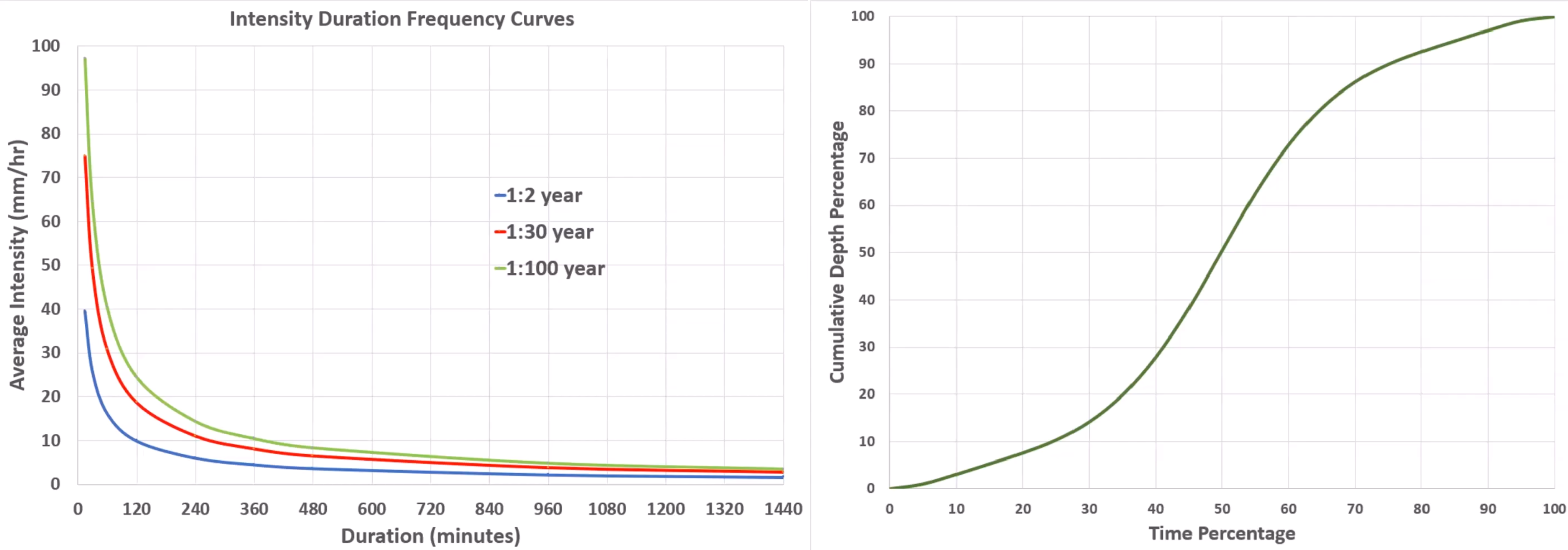
When working in a region that is not covered by one of the standard rainfall theories provided within the program, a rainfall definition can be built. This is done by entering two pieces of information: the IDF curve or curves, and the dimensionless shape curve.
First, create a new rainfall event:
- On the ribbon, Rainfall Pollutants tab, Rainfall panel, click Rainfall Manager.
- In the Rainfall Manager toolbar, click New.
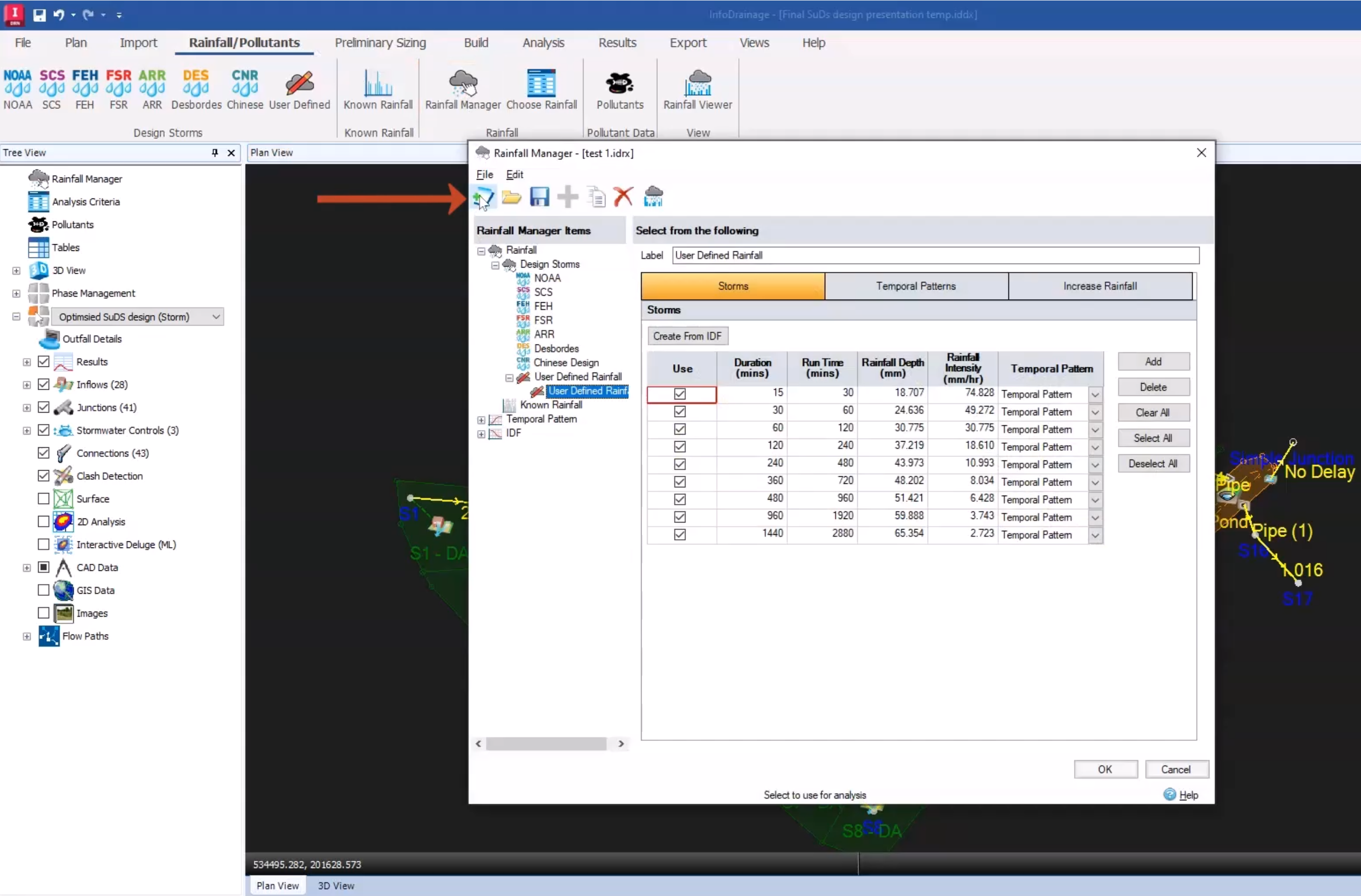
- Name the rainfall event. In this example, it is named “Test 1”.
- Click Save.
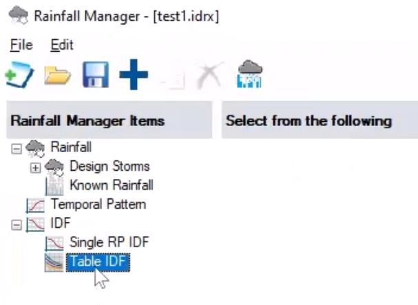
- Under Rainfall Manager Items, expand the IDF node to access the IDF library.
- Since this example uses a series of curves, select Table IDF to create a table of events. For a single curve, Single RP IDF would be selected.
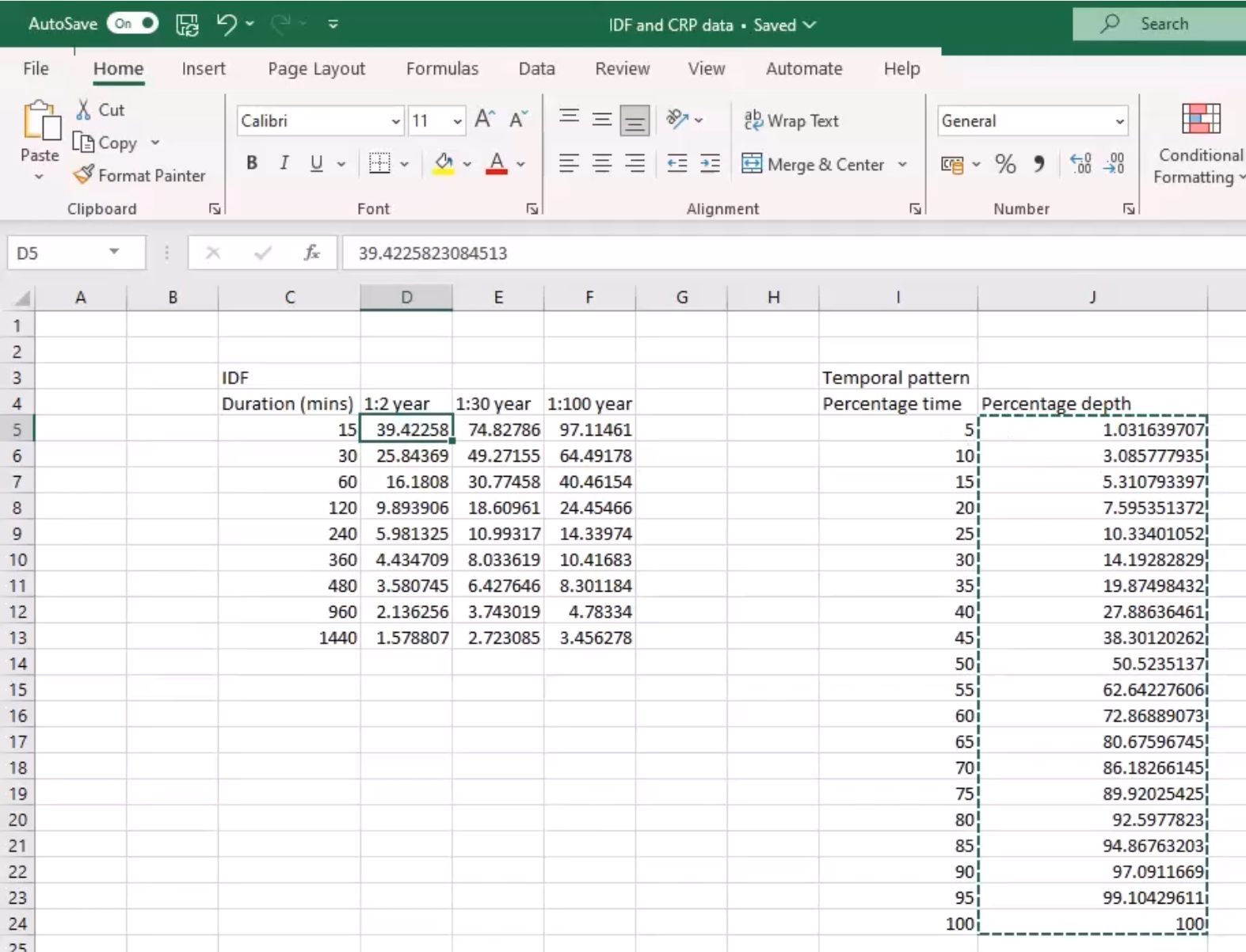
- Open the IDF and CRP data spreadsheet that contains the curve data.
This example uses data for the IDF curves for three storm durations, and temporal patterns for the dimensionless curve data. Start with the IDF data.
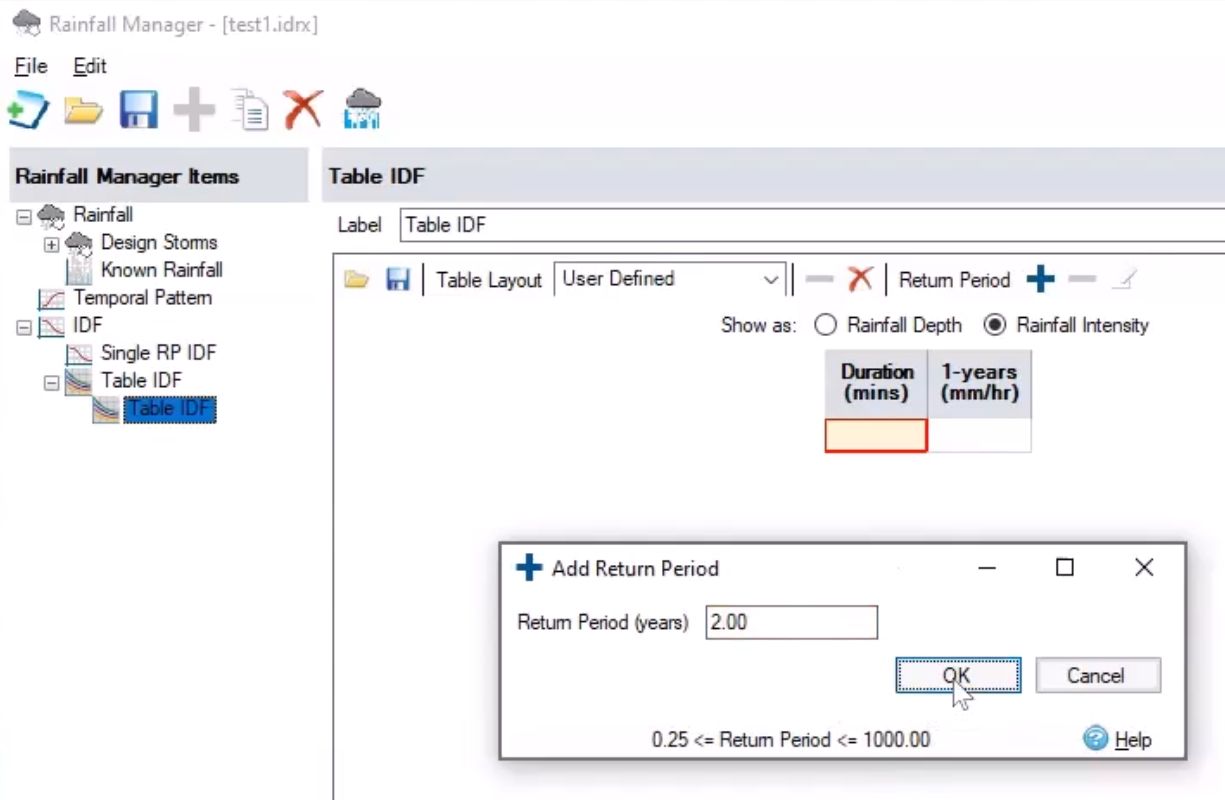
- In the Rainfall Manager, with Table IDF selected, click Add (+).
- Ensure that Rainfall Intensity is enabled.
Next, create columns for each of the three return periods:
- In the table tools, click Add (+).
- In the Add Return Period popup, in the Return Period (years) field, enter 2, for the 2-year return period.
- Click OK.
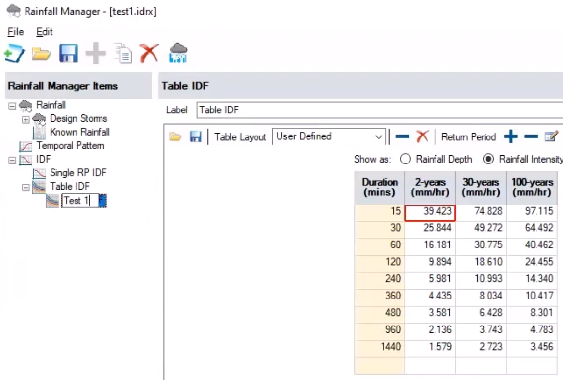
- Repeat steps 10 – 12 to add the 30-year and 100-year return periods.
To delete the 1-year return period, which is not needed for this example:
- In the Rainfall Manager table, select the 1-years (mm/hr) column header.
- Click Delete (-).
- In the IDF and CRP data spreadsheet, select the data, making sure not to include the headers.
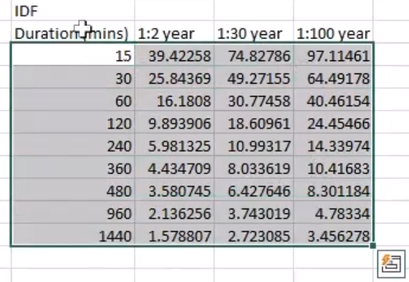
- Press Ctrl+C to copy the data to the clipboard.
- Back in the Rainfall Manager, in the table, click the first cell under Duration.
- Press Ctrl+V to paste the data.
- In the Items list, right-click the new Table IDF item and select Rename.
- Type “Test 1” to match the project name.
Next, enter the temporal pattern data, which again, is the dimensionless relationship data that defines the curve:
- In the Rainfall Manager Items list, click Temporal Pattern.
- In the toolbar, click Add (+).
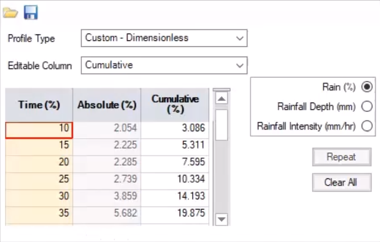
- Under Temporal Pattern, next to Label, enter a name, such as “Test 2”.
- Expand the Profile Type drop-down and select Custom – Dimensionless.
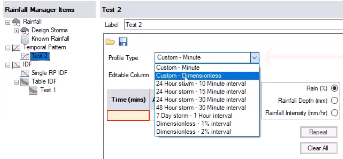
- Leave the Editable Column set to Cumulative.
- In the spreadsheet, select and copy the Percentage time values, from a non-zero value, such as 5, through 100.
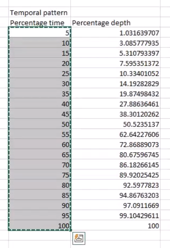
- In the Rainfall Manager table, under Time (%), paste the values.
- From the spreadsheet, copy the data under Percentage depth.
- In the table, under Cumulative (%), paste the values.
Now, bring the IDF curve and the shape of the event together to create a series of user-defined rainfall events.
- Under Rainfall Manager Items, expand the Design Storms node.
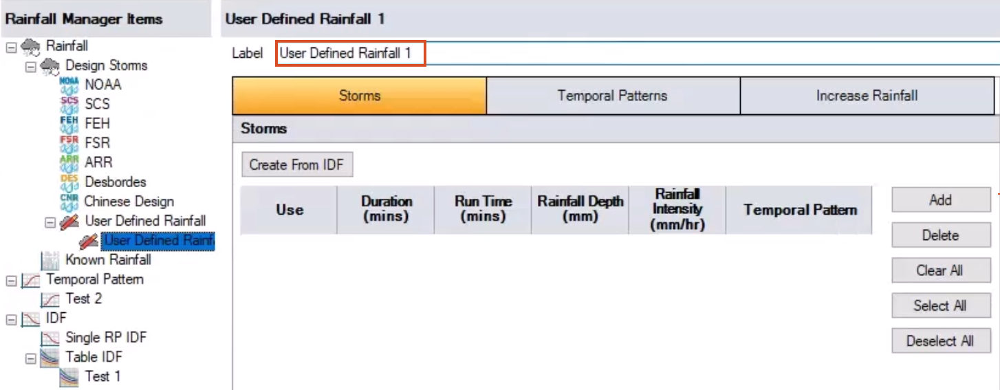
- Select User Defined Rainfall.
- Click Add (+).
- In the Label field, type “User Defined Rainfall 1” to rename it.
- Click OK to close the Rainfall Manager.
- Reopen the Rainfall Manager.
Closing and reopening the Rainfall Manager enables the library to update. The User Defined Rainfall 1 Design Storm remains active, and on the Storms tab, the Create From IDF tool is now available.
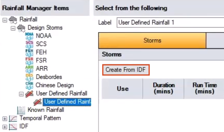
- Click Create From IDF.
- In the User Defined Rainfall From IDF popup, select From Library.
- Expand the drop-down and select the Test 1 IDF curve.
The return period information appears.
- Expand the Return Period drop-down and select 30-years.
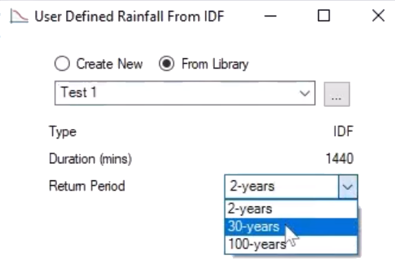
- Click OK.
- In the Label field, add “30 years” to the name for easier identification.
- Press ENTER to accept the change.
- In the table, in the Temporal Pattern column, expand each drop-down and select Test 2.
- Enable Use for all rows.
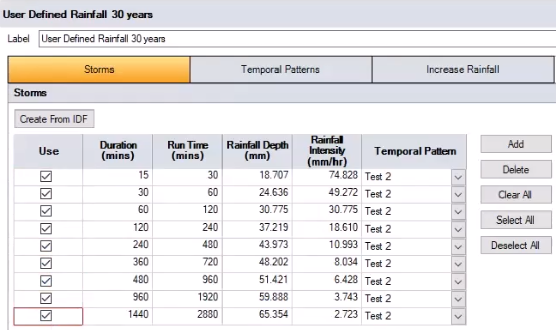
This means that these nine rainfall events will be used with the Temporal Pattern set to Test 2.
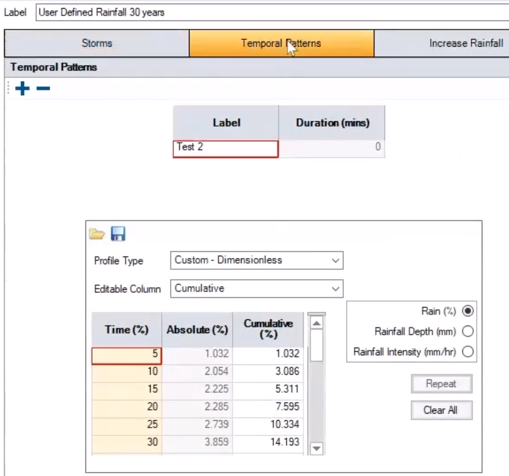
- Click the Temporal Patterns tab to double-check that it displays the data entered.
- Click the Increase Rainfall tab.
Adding in an aspect of climate change could be done here.
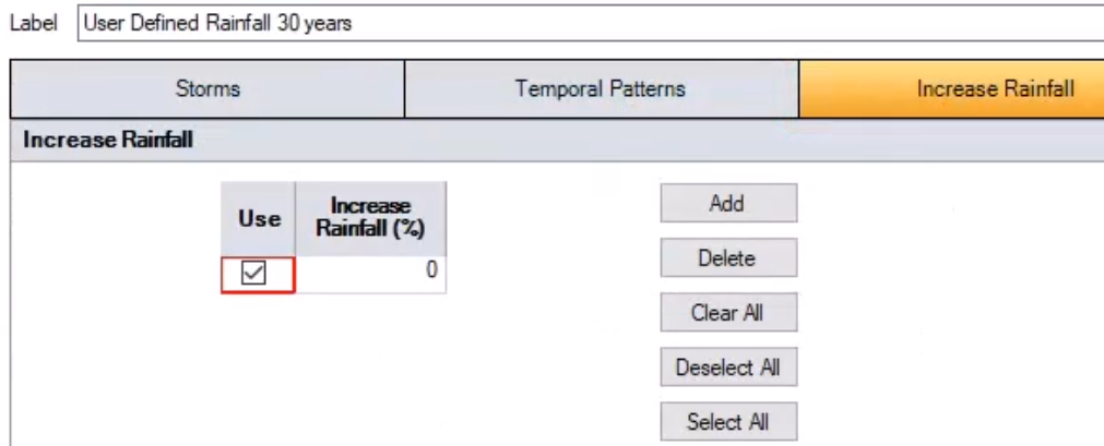
- Click Save to save the rainfall definition.
- Click OK to close the Rainfall Manager.
NOTE: this same rainfall later can be reused later, if needed.
Now, run an analysis using the data:
- On the ribbon, Analysis tab, Criteria panel, click Analysis Criteria.
In the Analysis Criteria dialog box, the User Defined Rainfall 30 years set of curves is now available, and crucially, there are nine rainfall events matching the nine chosen.
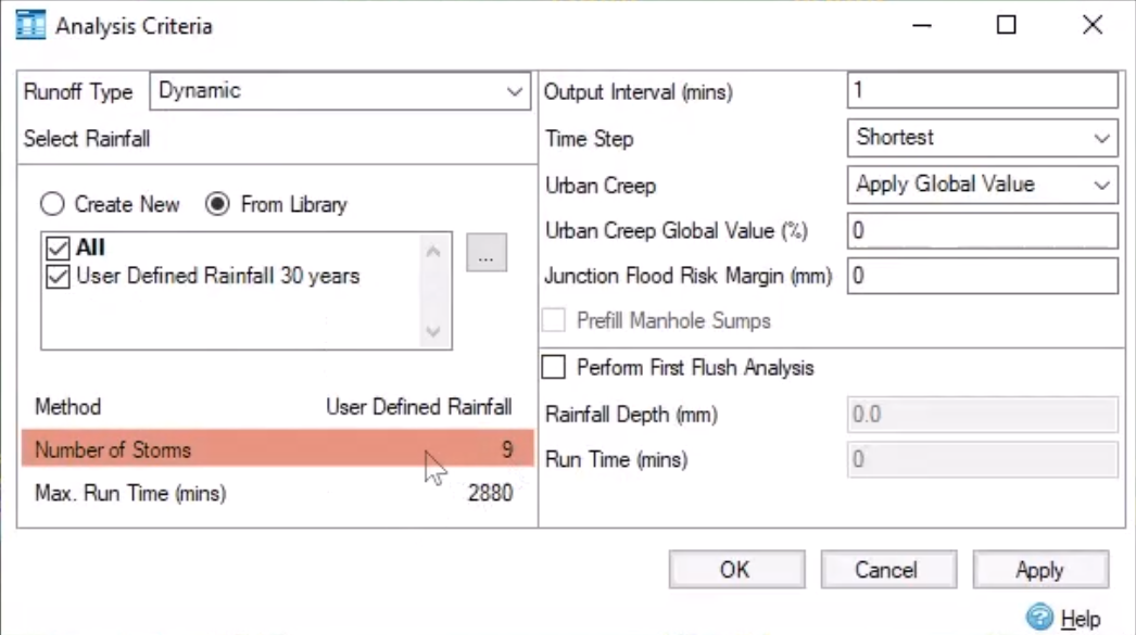
- Click OK.
- As a best practice, on the ribbon, click Validate.
- In the Validate dialog box, click OK.
- On the ribbon, click Go.
NOTE: Since the model used in this example is small—40 manholes and 40 pipes—and only 9 storms are used, this does not take long to process, but a larger model may take longer.
Once the simulation is finished, the Stormwater Controls Summary appears.
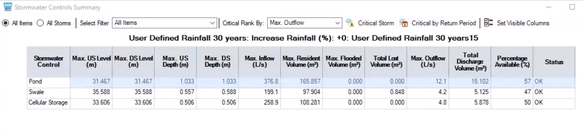
However, the results can be viewed in several different ways:
- Close the summary.
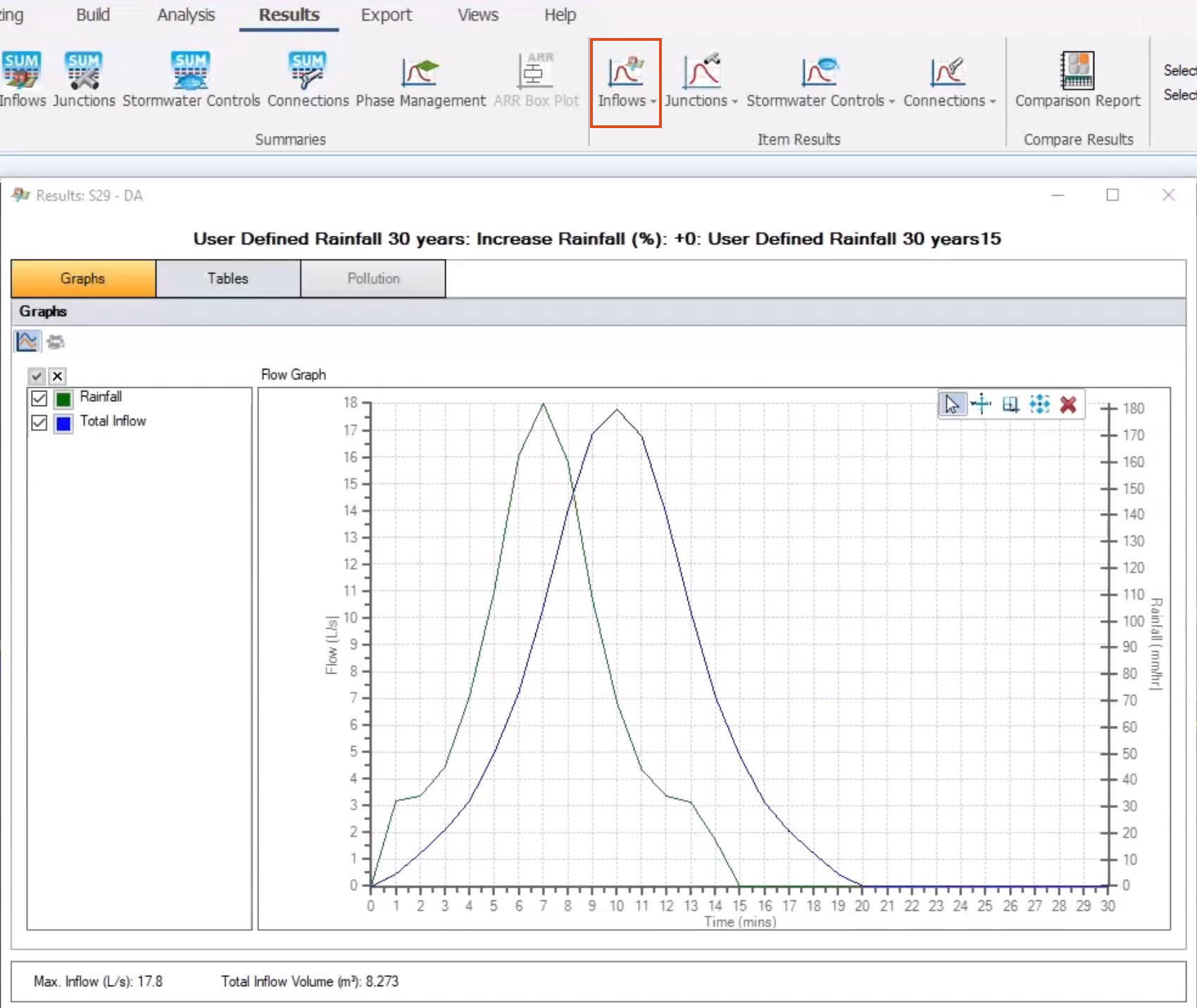
- On the ribbon, click the Results tab.
- As an example, in the Item Results, expand the Inflows drop-down and select S29-DA.
In the graph, flows entering or leaving an inflow area, or flows entering a manhole can be reviewed. Specific rainfall events can also be selected.
- In the Event Selection panel, expand the Select Event drop-down and choose a different rainfall event, such as 240.
- In the graph, deselect the Total Inflow to see only the Rainfall.
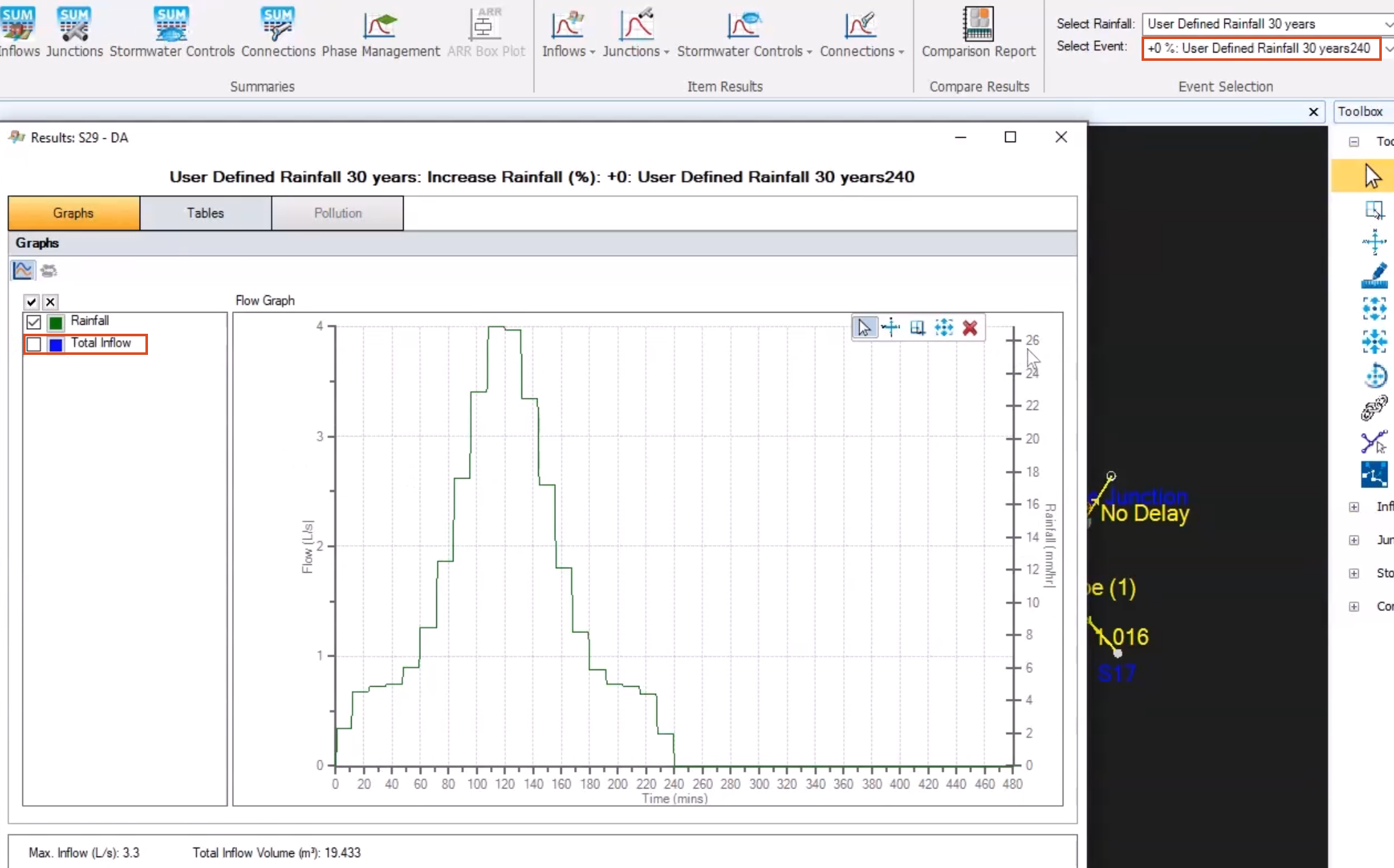
In this case, because it is a 1-in-30-years storm, 240-minute event, the maximum intensity is a little more than 26 millimeters per hour.
Creating rainfall data for determining temporal patterns is a straightforward process, provided the IDF curve and shape curve data for the area of interest is available.


