00:03
InfoSurge Pro allows you to create hydraulic transients by providing a curve which will alter pump and valve operations,
00:10
as well as junction demand changes.
00:13
You can then compare the simulation results from different operational conditions.
00:18
In this example, you create transient events from valve operations.
00:23
To begin, double-click the desired project .aprx file to open ArcGIS Pro.
00:29
Once the project starts, click the InfoWater Pro tab to open the InfoWater Pro ribbon.
00:35
In the Project panel, click Initialize.
00:38
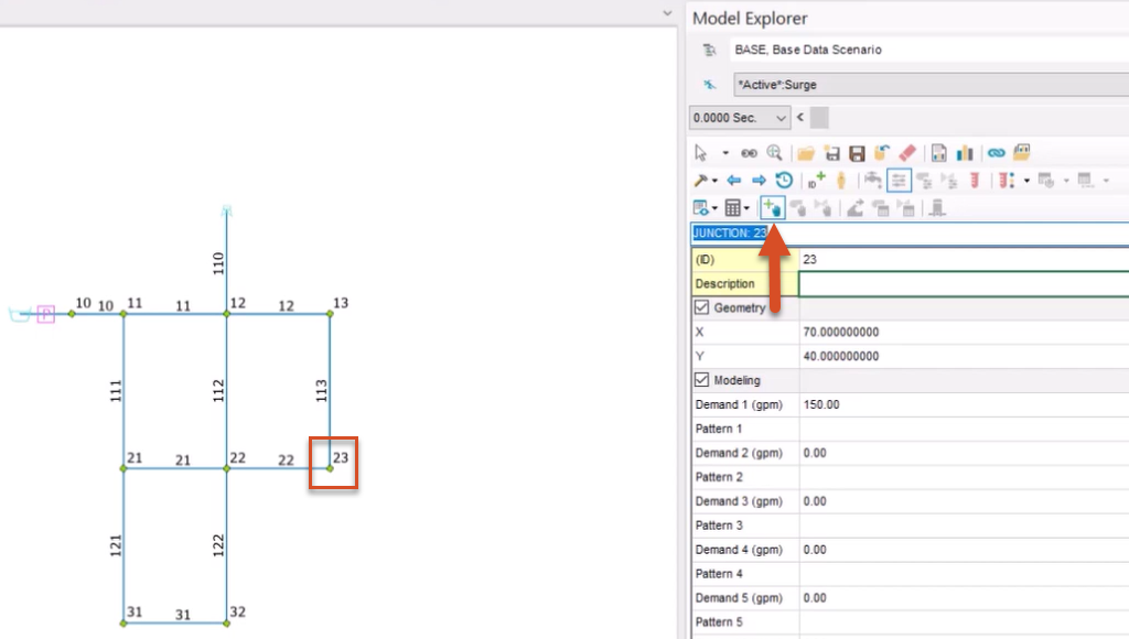
From the map, select Junction 23.
00:42
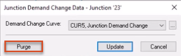
Then, from the Model Explorer, click the Demand Change button to open the Junction Demand Change Data dialog.
00:49
Click Purge to remove all existing settings.
00:52
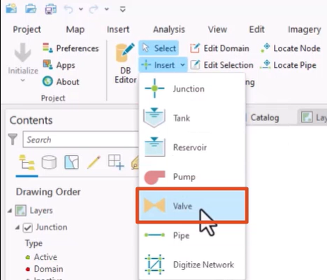
Next, create a valve.
00:54
From the ribbon, InfoWater Pro tab, Edit panel, expand the Insert drop-down and pick Valve.
01:02
Click the middle of Pipe 111.
01:06
In the notification asking if you want to insert a valve on the pipe, pick Yes.
01:12
In the Valve Identification dialog, Valve ID field, enter “V1”,, and then click OK to generate a new valve (V1) and a new pipe (P11).
01:23
From the ribbon, InfoWater Pro tab, Edit panel, click the Select tool to enable it.
01:29
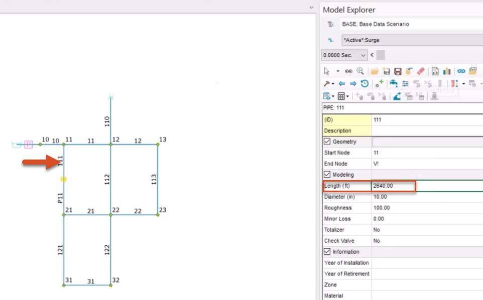
Then, click Pipe 111.
01:32
From the Model Explorer window, change the Length of the pipe to 2640 feet, or half of the original length.
01:39
Change the Length of pipe P11 to match.
01:44
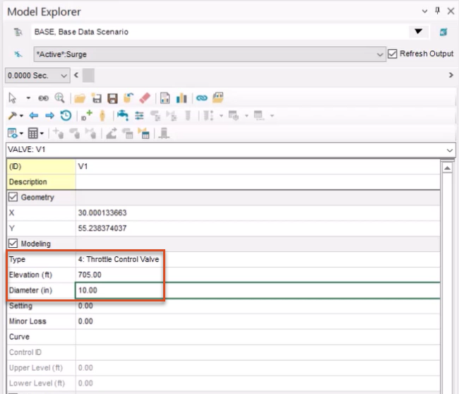
Now, select valve V1.
01:47
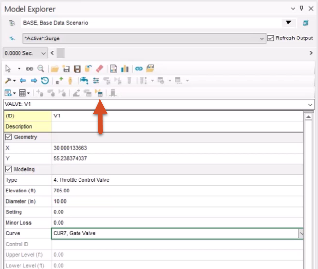
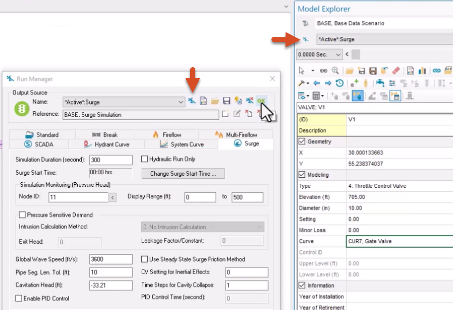
From the Model Explorer, change the valve Type to 4: Throttle Control Valve.
01:54
Set the Elevation to 705 feet, and the Diameter to 10 inches.
01:60
Any change in valve position (% open) will produce a transient.
02:05
To model this based on valve operation, two curves would need to be assigned.
02:10
The first is the Active Valve Characteristic curve, which represents the “% stem position” vs. the “minor loss K”.
02:18
These correspond with the percentage open the valve is (10 = 10% open)
02:23
and the minor loss coefficient that accounts for energy lost from flow through the valve.
02:28
The second is the Operational Change Data curve, which describes “time” vs. “% stem position”.
02:35
These curve parameters would show the change in how open the valve is (% open) over time.
02:42
Together, these two curves account for the valve characteristics
02:45
and the change in stem position during the transient analysis, respectively.
02:49
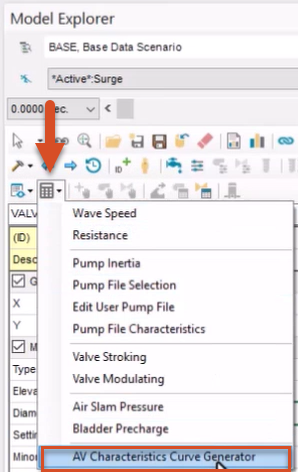
To calculate the valve characteristics curve, from the Model Explorer, click the Auxiliary Calculator button,
02:56
and in the drop-down, pick AV Characteristics Curve Generator.
02:60
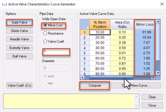
In the Active Valve Characteristics Curve Generator dialog, in the Options group box, click Gate Valve.
03:07
In the Pipe Data group box, enable the Minor Loss option and enter a value of “1” in the blank text box.
03:14
Then, click Compute to calculate the active valve curve.
03:18
Note that the Minor Loss K column populates with calculated data.
03:23
Next, click Create New Curve to open the New Curve dialog.
03:27
In the New ID field, type a name for the new curve.
03:31
In this example, the name “CUR7, Gate Valve” is entered.
03:38
Note that in the Active Valve Characteristics Curve Generator dialog, a message reads:
03:44
“Curve CUR7 has been inserted into your DB tables.”.
03:50
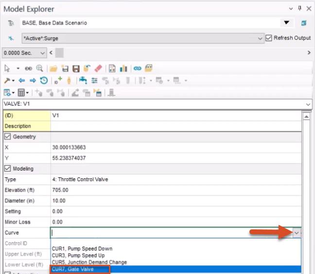
Now, select valve V1.
03:53
From the Model Explorer, in the Curve field drop-down, select CUR7, Gate Valve.
03:60
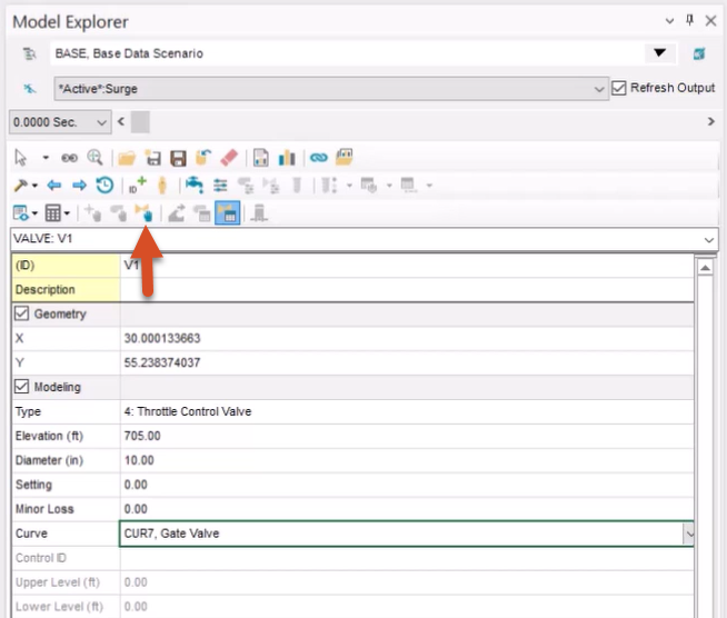
Then, click the AV (TCV) Surge Data button.
04:04
The throttle control valve must be identified as an active valve to use during the surge analysis.
04:10
If required, a bypass line or check valve can be added in this dialog as well, however they will not be used in this example.
04:18
In the Active Valve Data dialog, click Activate to activate the valve.
04:23
You are now ready to create the Operational Change Data curve for the valve.
04:28
From the Model Explorer, click the AV (TCV) Operation Change button.
04:33
This button would not be available if the valve had not been activated.
04:37
In the dialog that opens, next to the Stem Change Curve drop-down, click Browse to open the Curve dialog.
04:44
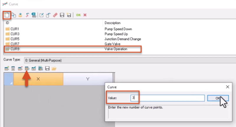
Click New to create a new stem change curve.
04:48
Give the new curve an ID of “CUR9, Valve Operation”, and then click OK.
04:55
Next, pick the Set Rows button, and in the Curve popup, assign a Value of “3”.
05:02
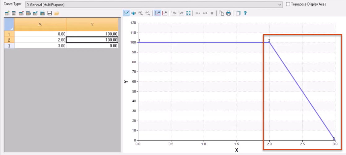
In the table, enter the following values by assigning each X-axis value (time in seconds) in numerical order,
05:09
followed by the values in the Y-axis column (valve % open).
05:14
In the X-column, enter: 0.00 in row 1
05:25
In the Y-column, enter: 100.00 in row 1
05:36
The graph shows that after the first two seconds, the valve will turn from fully open to fully closed within the next one second.
05:43
Click OK to close the dialog, and then click Create in the remaining dialog.
05:49
Now, from the Model Explorer, click the Run Manager button.
05:53
Or, from the ribbon, Analysis panel, click the Run button.
05:57
In the Run Manager dialog, click the Run button to run a surge analysis.
06:03
Click OK to close the dialog.
06:06
Then, from the ribbon, View panel, click Report Manager.
06:10
In the Report Manager dialog, click New, and under Available Output Sources, select *Active*.Surge.
06:19
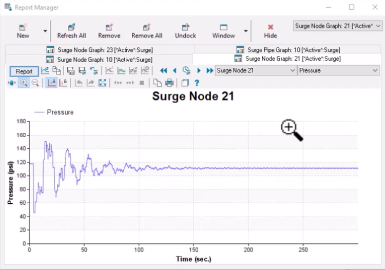
From the Graph Report tab, select Surge Node Graph, then click Open.
06:24
From the map, select Junction 21 to view its pressure profile.
06:29
Note that closing the valve within one second did create a transient event.
06:35
To see how the profile changes with a longer valve operation time, click the AV (TCV) Operation Change button.
06:42
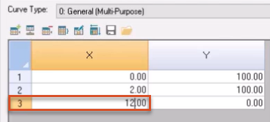
Reopen the Curve dialog, and in the table, X-column, change the value in the third row to 12.00.
06:51
This extends the valve closure time from one to 10 seconds.
06:56
Click OK, and then Update.
06:60
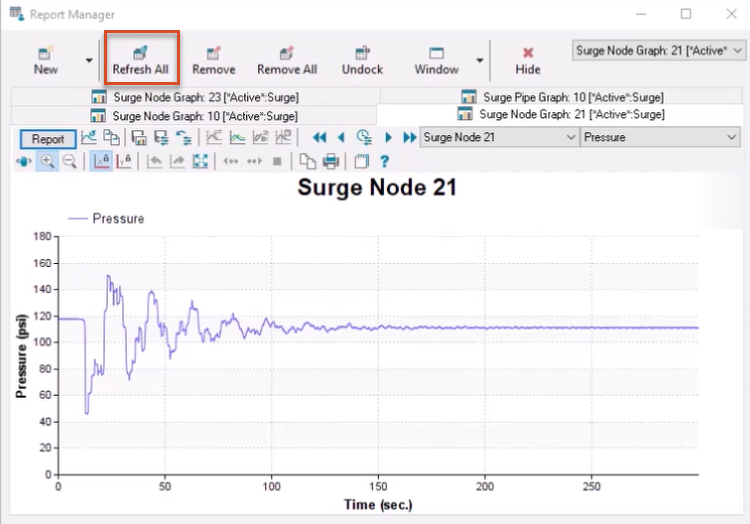
Reopen the Run Manager, run another surge analysis, and then close the dialog.
07:08
Reopen the Report Manager, and then click Refresh All to view the new output results.