00:03
InfoSurge Pro allows you to create hydraulic transients by providing a curve which will alter pump and valve operations,
00:11
as well as junction demand changes.
00:13
You can then compare the simulation results from different operational conditions.
00:18
In this example, transients are created from pump shutdown events using the Pump Speed Change option.
00:25
To begin, double-click the desired project .aprx file to open ArcGIS Pro.
00:32
Once the project starts, click the InfoWater Pro tab to open the InfoWater Pro ribbon.
00:38
In the Project panel, click Initialize.
00:41
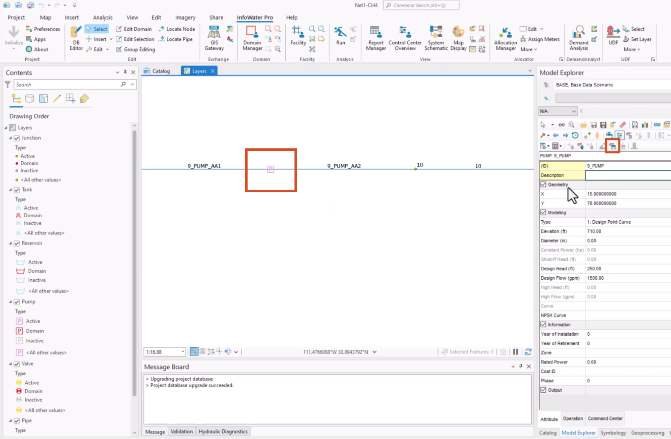
Next, with the Select tool active, zoom to and select the pump with the ID 9_PUMP.
00:48
From the Model Explorer, click the Pump Surge Data button.
00:53
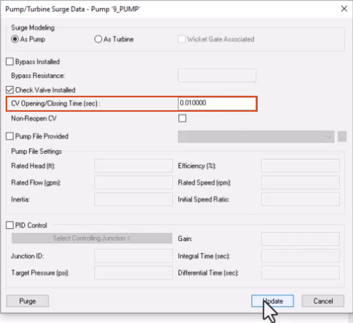
The Pump Surge Data dialog box is used to specify how the selected pump and its associated properties will be modeled.
01:01
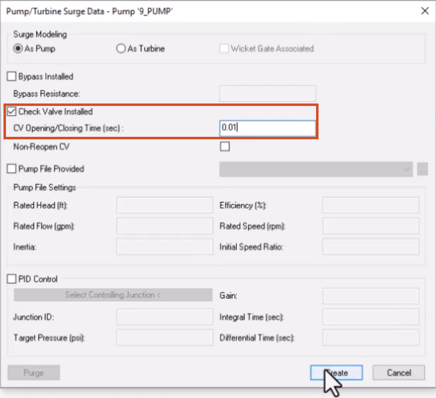
First, make sure a check valve is modelled for the surge analysis by enabling the Check Valve Installed option.
01:08
This will prevent flow reversal through the pump.
01:12
Enter a check valve (CV) opening and closing time of 0.01 seconds.
01:19
Then, click Create to save the settings and close the dialog.
01:24
Changes in pump operating speeds produce transients.
01:28
Time-dependent speed ratios can be applied to pumps as a speed curve.
01:33
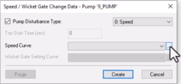
To do so, from the Model Explorer, click the Pump Operation Change button.
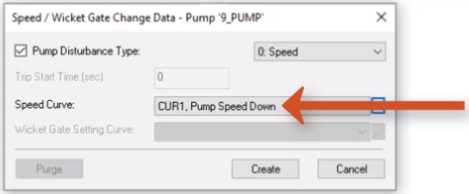
01:38
In the Pump Operation Change dialog, select the Pump Disturbance Type option,
01:43
and then set the disturbance speed to “0: Speed”.
01:47
The curve selected will dictate the pump speed over time.
01:51
Next to the Speed Curve drop-down, click the Browse (...) button.
01:55
This opens the Curve dialog.
01:57
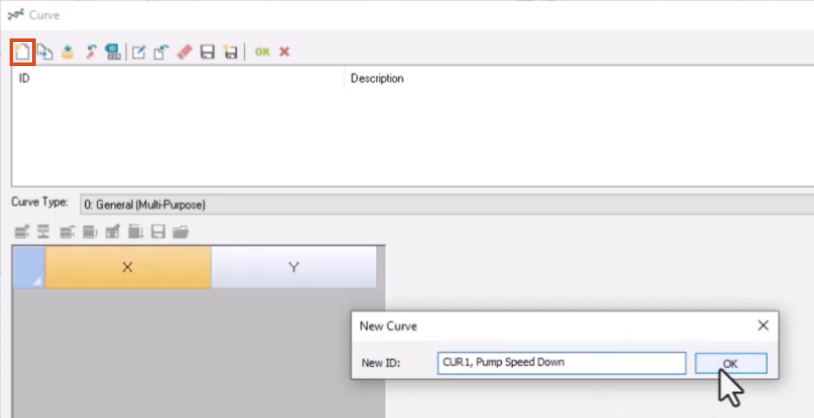
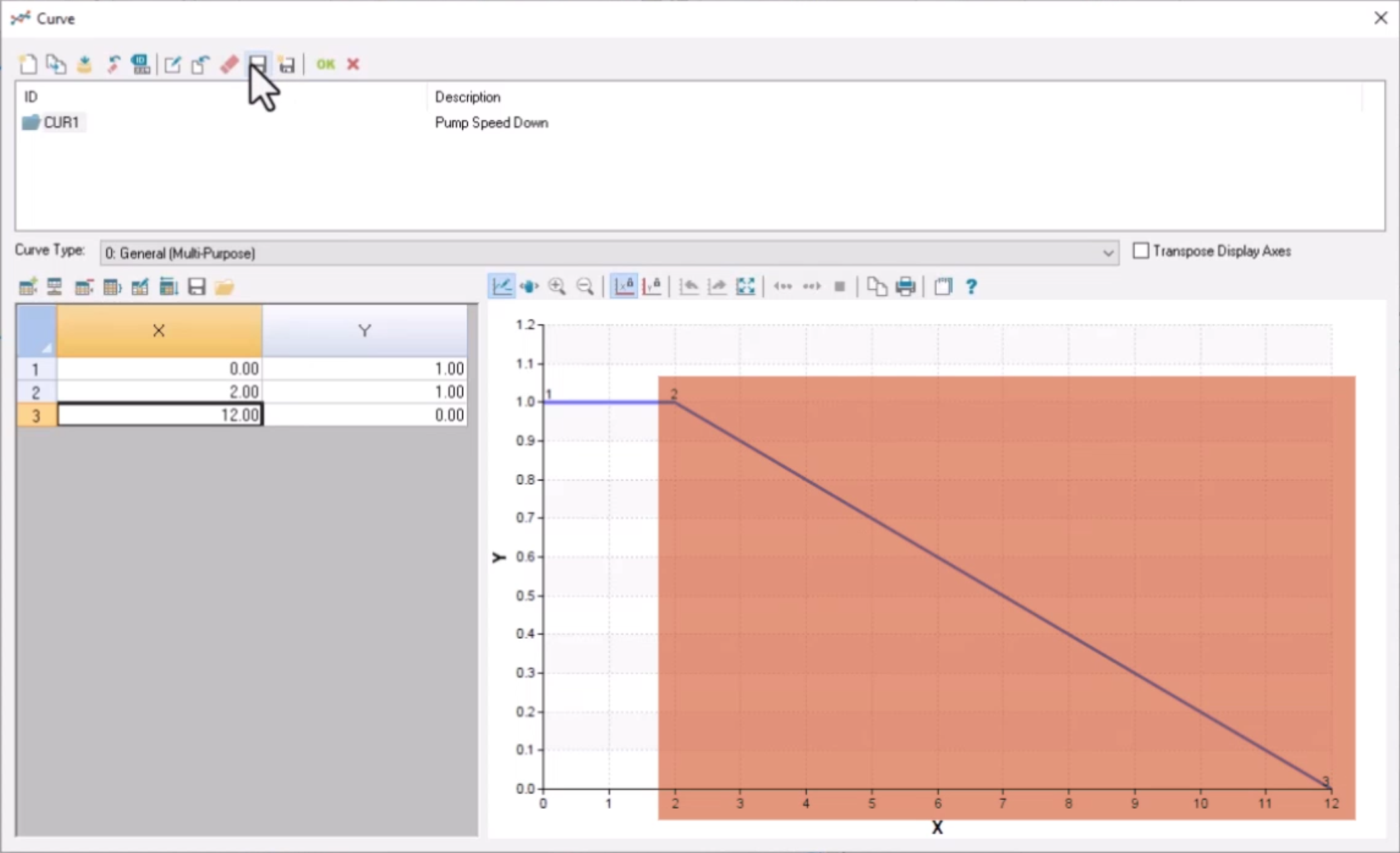
The model does not currently have a speed curve to use, so one must be created.
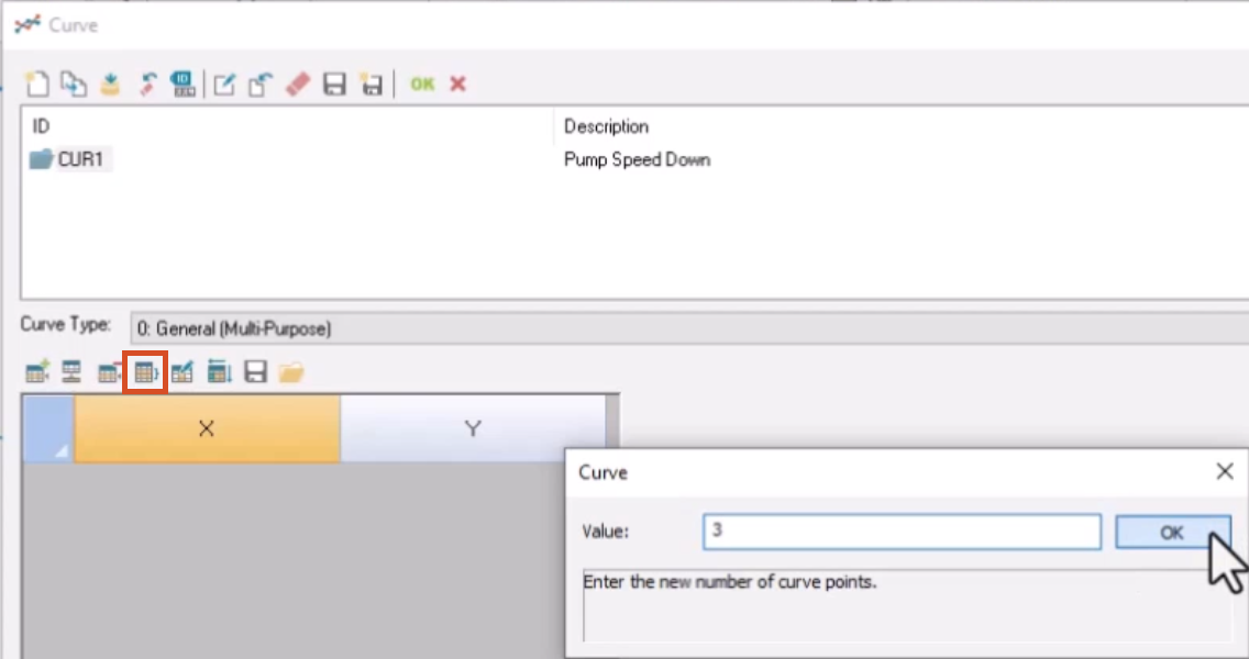
02:02
Click the New icon, and you are prompted to name the new curve ID.
02:06
Enter the name “CUR 1, Pump Speed Down”, and then click OK.
02:12
With the Curve dialog still open, click the Set Rows button.
02:16
In the Value field, enter “3”, and then click OK.
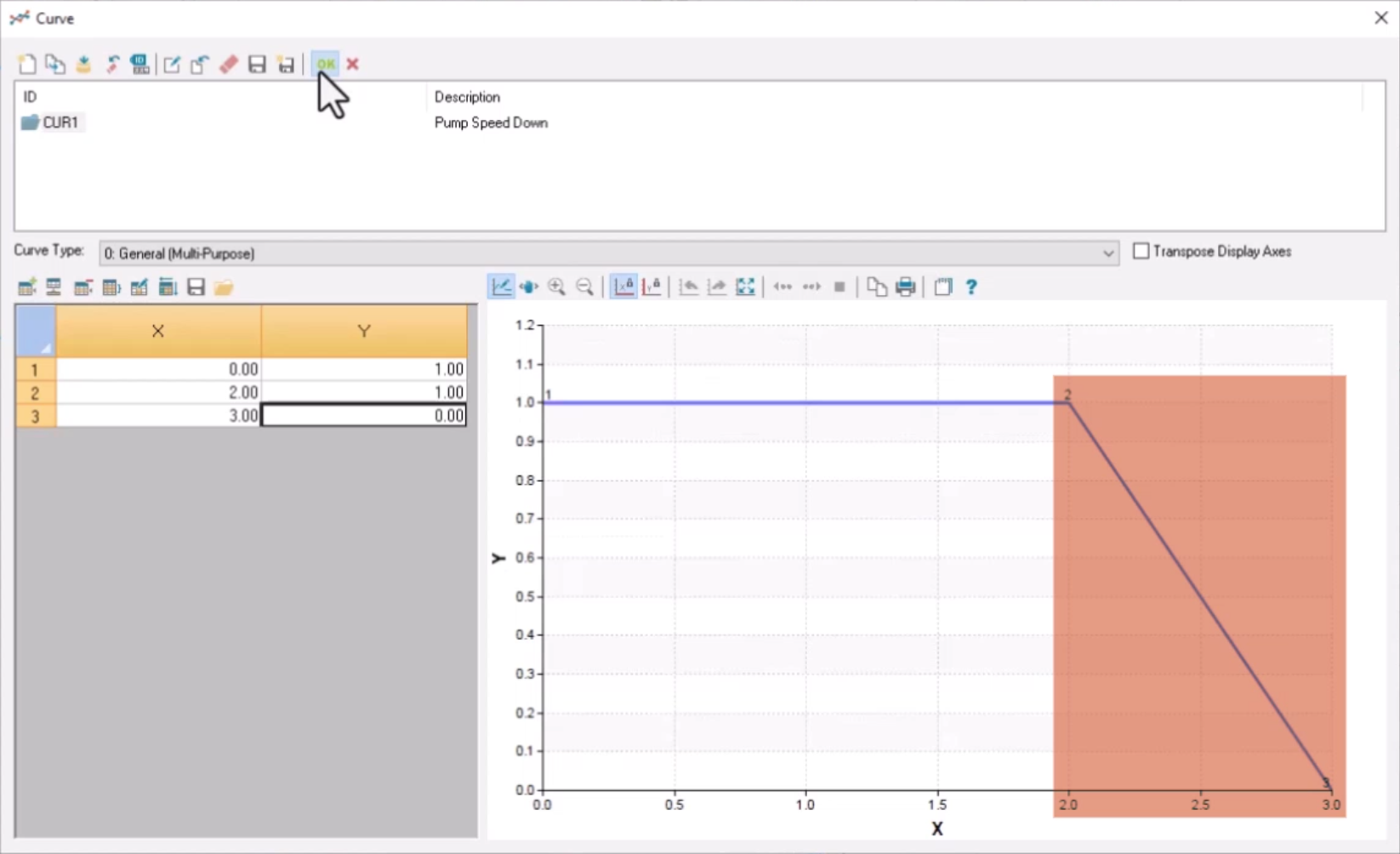
02:21
The X/Y table updates to have three rows and two columns.
02:26
You can now enter values into the table to create a pump curve, which updates automatically in line graph form.
02:33
Note that the X-axis is operation time in seconds,
02:36
and the Y-axis represents pump speed ratio.
02:40
Enter the following values by assigning each X-axis value in numerical order,
02:45
followed by the values in the Y-axis column.
02:49
In the X column, enter: 0.00 in row 1
03:01
In the Y column, enter:
03:12
Note that the curve indicates that after two seconds, the pump will drop from full speed (1 for 100% speed)
03:19
to off (0 for 0% speed) within the next one second.
03:24
Click OK to close the Curve dialog.
03:27
In the Speed/Wicket Gate Change Data dialog, make sure the Speed Curve drop-down is set to the name of the new curve you just created.
03:35
Then, click Create to close the dialog and save the settings.
03:40
You are now ready to run both steady-state and surge simulations.
03:45
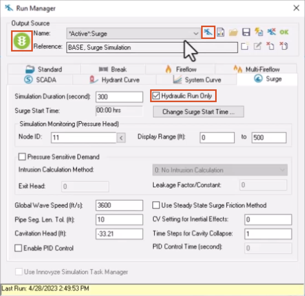
From the Model Explorer, click the Run Manager button,
03:48
and then, in the Run Manager, open the Surge tab.
03:52
Enable the Hydraulic Run Only option, and then click Run to run the model with a hydraulic simulation.
03:59
Upon successful completion, under Output Source,
04:02
a green light icon appears, and you are ready to run a surge analysis.
04:07
Deselect the Hydraulic Run Only option, and then click Run again to perform a surge analysis.
04:14
Click OK to close the Run Manager.
04:17
If you are prompted about switching to the most recent run output data, select Yes.
04:23
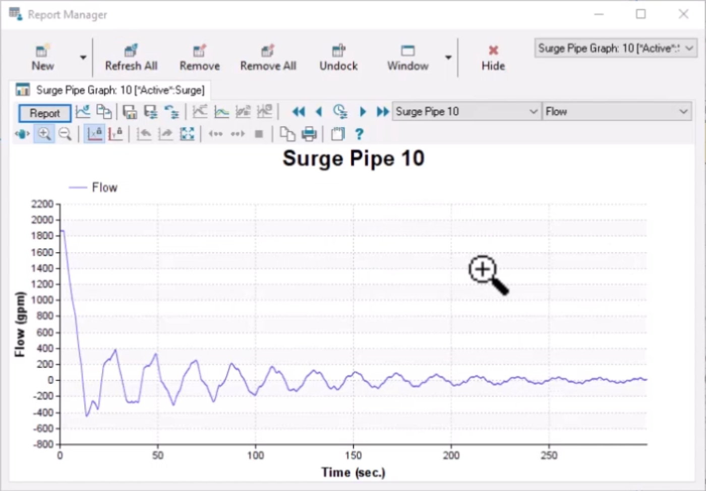
Results from the simulation can be viewed in graph or tabular format.
04:28
For this example, you will view the effect of the surge simulation on flow through a pipe downstream of the pump experiencing
04:37
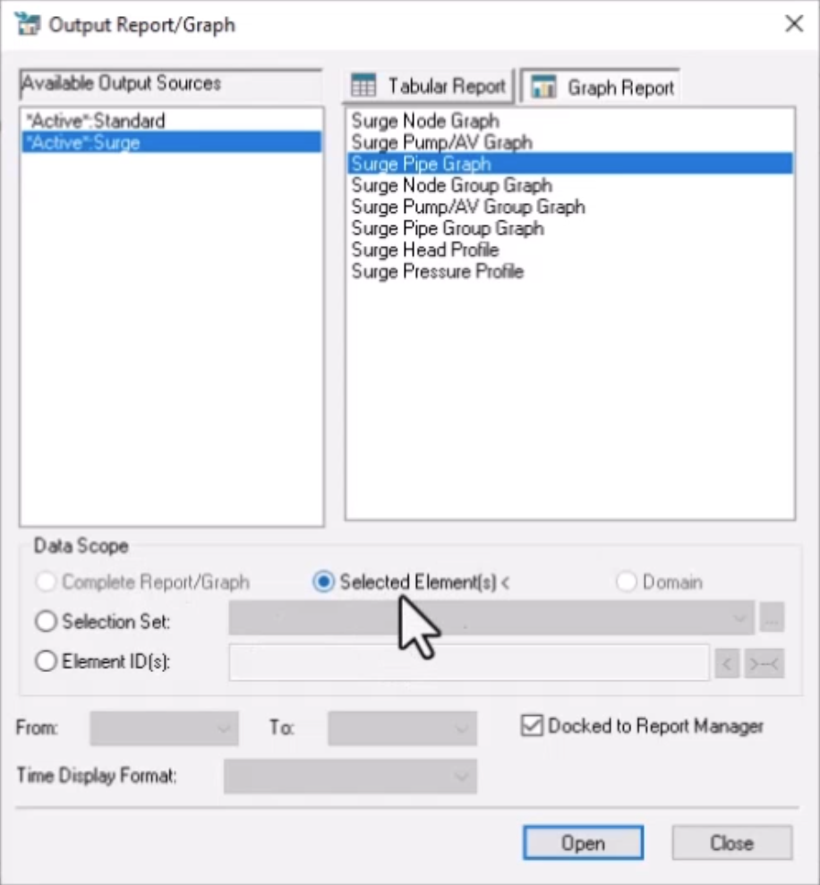
From the ribbon, InfoWater Pro tab, View panel, click Report Manager.
04:42
In the Report Manager dialog, click the New button to open the Output Report/Graph dialog.
04:49
Under Available Output Sources, select *Active*.Surge.
04:53
Then, open the Graph Report tab and select Surge Pipe Graph.
04:58
Note that in the Data Scope group box, the default option Selected Element(s) is enabled.
05:06
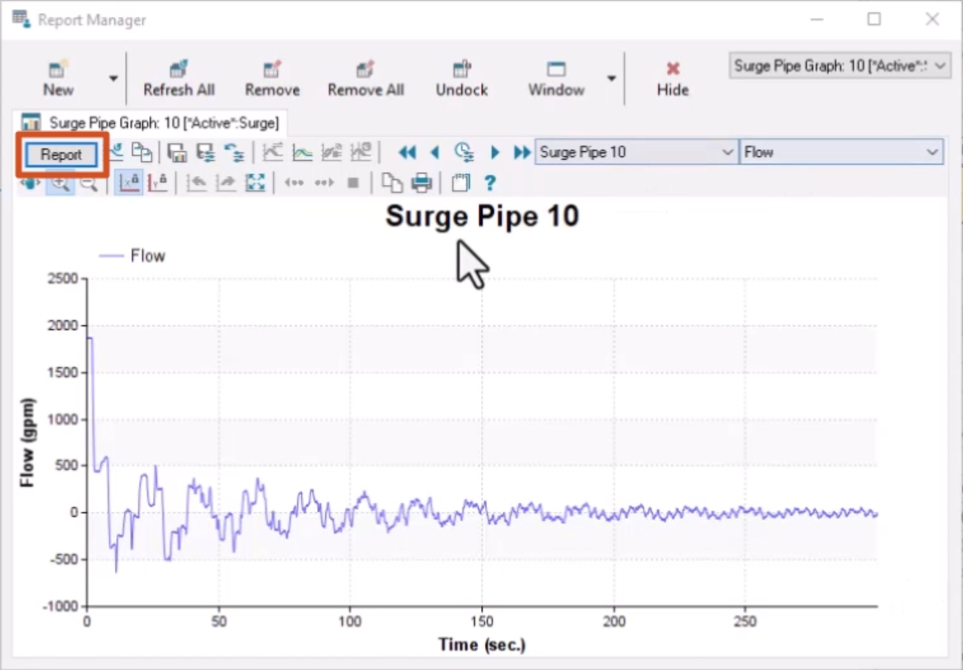
On the map, select Pipe 10 to view its flow, which indicates a typical pump shutdown response.
05:12
Review the graph and, if needed, click Report to see data for the entire run in a table format.
05:20
Close out of the Report Manager once you are done reviewing.
05:24
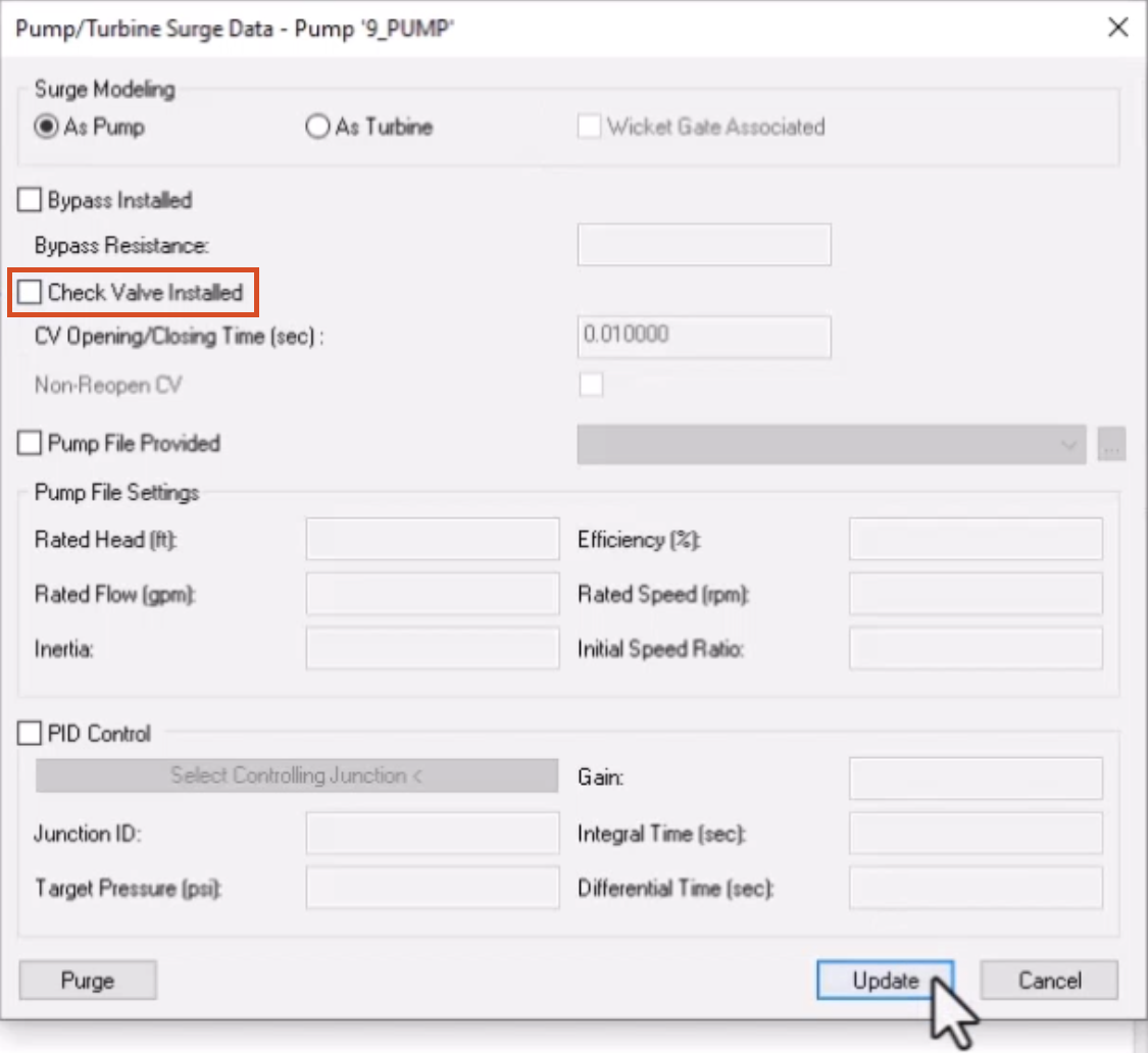
The previous results can be compared to a new simulation that is run without a check valve
05:28
to better understand the effects of modelling a check valve in your system.
05:36
Click the Pump Surge Data button to open the Pump/Turbine Surge Data dialog.
05:41
Disable the Check Valve Installed option, and then click Update.
05:46
Next, reopen the Run Manager.
05:49
Click the Run button to run a surge analysis.
05:53
Then, click OK to close the dialog.
05:57
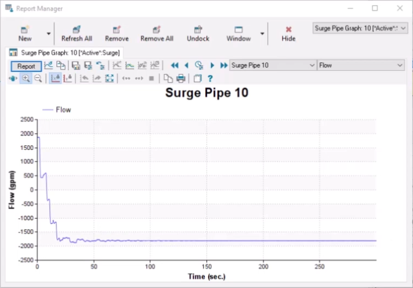
Reopen the Report Manager and click Refresh All.
06:01
This refreshes the output for pipe 10 for the latest run.
06:05
You can now review the results using the Report Manager.
06:08
Notice the difference in flow from the previous run as a result of removing the check valve.
06:14
Without the check valve to prevent reverse flow, additional flow can go through the pipe.
06:19
When you finish reviewing the results, Close the Report Manager.
06:23
Shorter shutdown times are going to create greater surge events,
06:27
whereas a slower shutdown will produce less of a transient event.
06:32
For the next step, you use a longer pump speed change operation time
06:36
to increase the pump shutdown time and minimize the impact of the surge event.
06:41
From the map, select pump 9_PUMP.
06:45
Click the Pump Surge Data button, and then in the Pump Surge Data dialog,
06:49
enable the Check Valve Installed option.
06:52
Note that the software should remember the previously entered CV closing time,
06:56
so leave it set to 0.01 seconds.
07:02
From the Model Explorer, click the Pump Operation Change button to open the Speed/Wicket Gate Change Data dialog.
07:09
Then, click Browse (...) to reopen the Curve dialog.
07:13
Make sure the CUR1 curve ID is selected.
07:17
Then, in the X-column, set the value in row 3 to 12.00.
07:22
This greatly extends the pump speed downtime from one second to ten seconds.
07:28
Click Save to save the changes, and then OK to close the dialog.
07:33
In the remaining dialog, click Update to update the changes and close the window.
07:38
Reopen the Run Manager and select Run to begin a surge analysis.
07:43
Reopen the Report Manager and click Refresh All to refresh the output for pipe 10 for the latest run and view the results.
07:51
Notice the surge event is greatly reduced.
07:54
This process could be repeated with different shutdown times to identify how slow pump shutdown would need to be
08:00
to avoid a surge event.