00:03
InfoSurge Pro allows you to create hydraulic transients by providing a curve which will alter pump and valve operations,
00:10
as well as junction demand changes.
00:13
You can then compare the simulation results from different operational conditions.
00:18
In this example, you create transients from junction demand changes.
00:22
To begin, double-click the desired project .aprx file to open ArcGIS Pro.
00:29
Once the project starts, click the InfoWater Pro tab to open the InfoWater Pro ribbon.
00:35
In the Project panel, click Initialize.
00:38
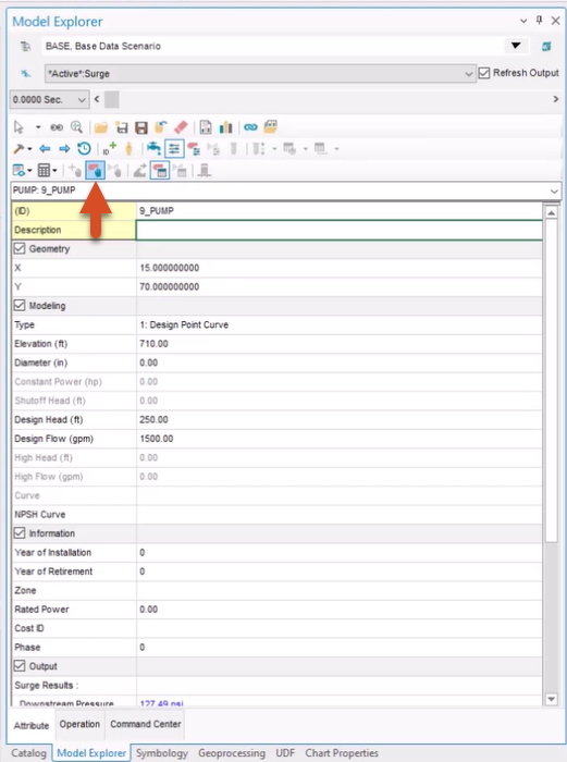
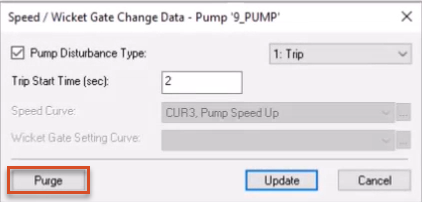
From the Model Explorer, select Pump Operation Change.
00:42
In the Speed/Wicket Gate Change Data dialog, click Purge to remove all previously entered settings.
00:49
Next, create a curve to describe the junction demand over time.
00:54
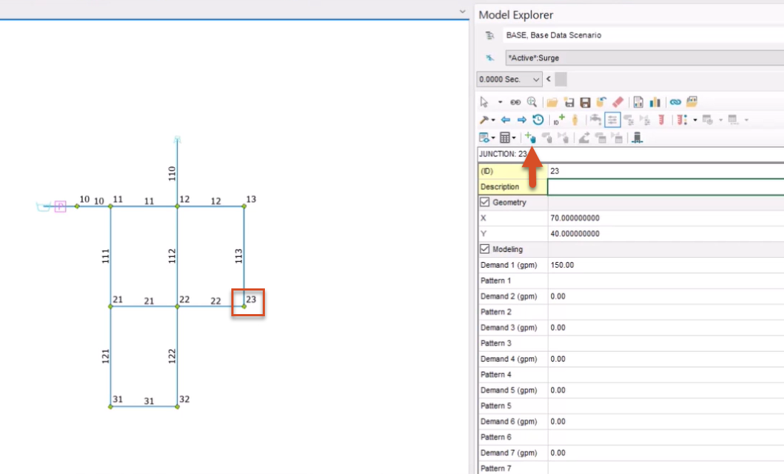
For this example, use Junction 23.
00:57
From the map, zoom to and select Junction 23.
01:02
With the junction selected, from the Model Explorer, click the Demand Change button.
01:08
In the Junction Demand Change Data dialog, next to the Demand Change Curve drop-down, click Browse (…) to open the Curve dialog.
01:17
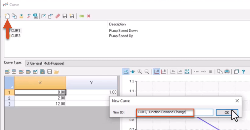
Click New to create a new junction demand change curve.
01:21
In the New ID field, enter “CUR5, Junction Demand Change” and then click OK.
01:27
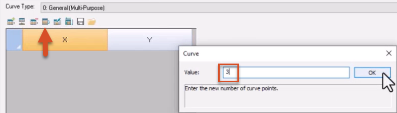
Now, click the Set Rows button.
01:30
Set the value to 3, and then click OK.
01:34
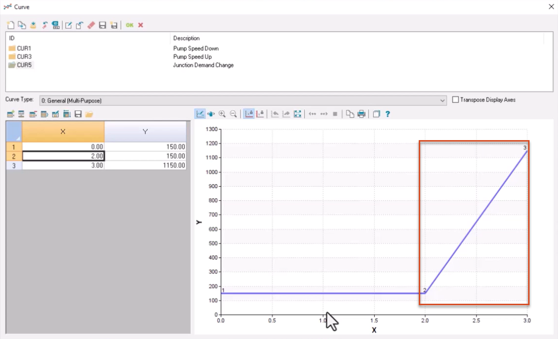
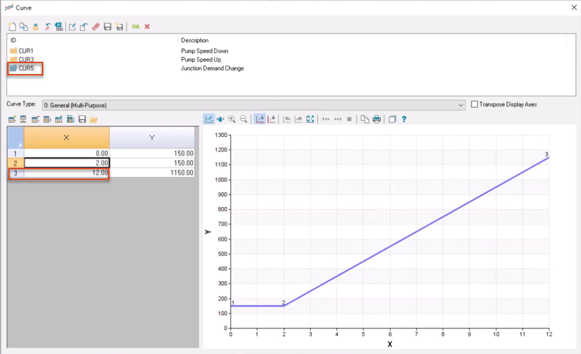
In the table, enter the following values by assigning each X-axis value (time in seconds) in numerical order,
01:41
followed by the values in the Y-axis column (demand in gallons per minute).
01:46
In the X-column, enter: 0.00 in row 1
01:58
In the Y-column, enter: 150.00 in row 1
02:11
Note that the updated graph indicates that after the first two seconds,
02:15
the demand will increase from 150 to 1150 gallons per minute in one second.
02:21
Such a demand increase may indicate fire flow.
02:24
Click OK, and then, in the remaining dialog, select Create.
02:29
You are now ready to perform a surge analysis.
02:33
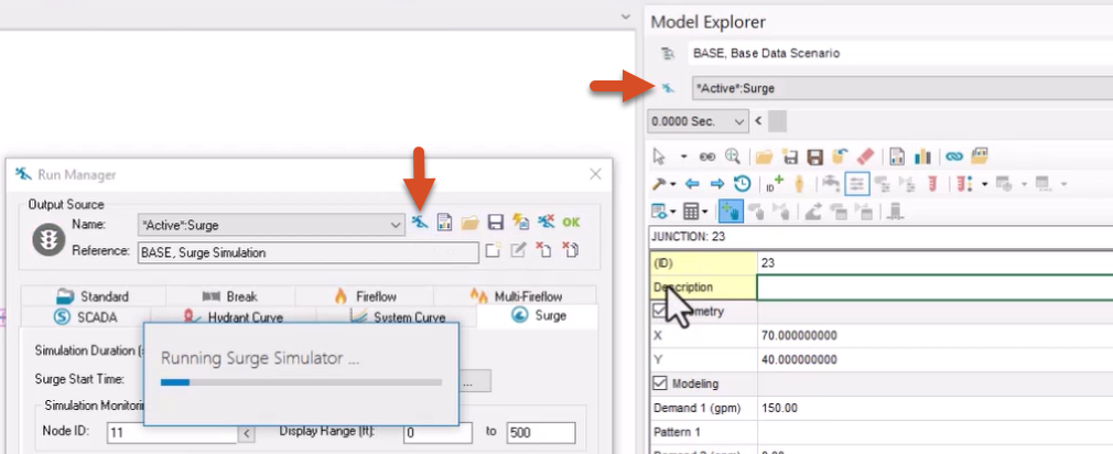
From the Model Explorer, click the Run Manager button.
02:37
Or, from the ribbon, InfoWater Pro tab, Analysis panel, click Run.
02:42
In the Run Manager dialog, click the Run button to perform a surge analysis, then click OK to close the dialog.
02:50
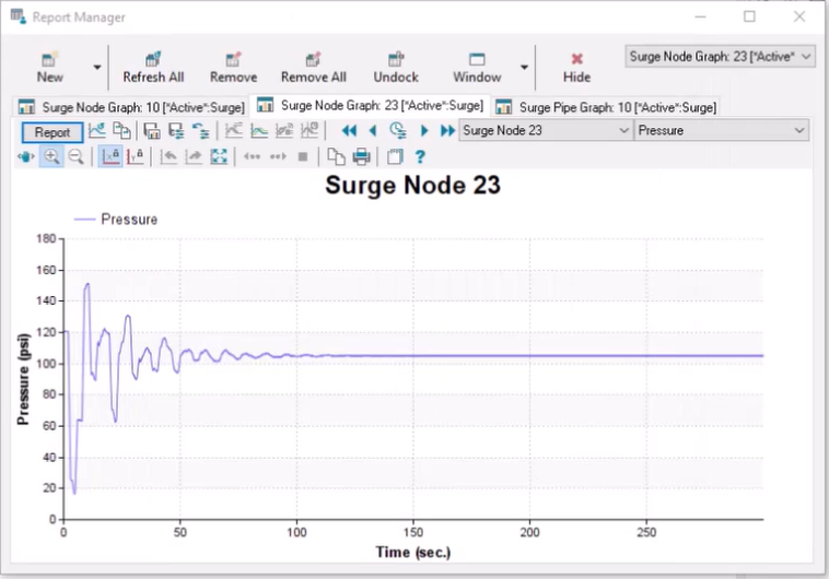
From the ribbon, View panel, click Report Manager.
02:55
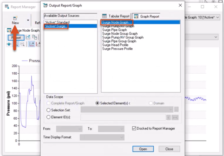
In the Report Manager dialog, click New.
02:59
In the Output Report/Graph dialog, under Available Output Sources, make sure *Active*.Surge is selected.
03:07
From the Graph Report tab, pick Surge Node Graph, and then click Open.
03:12
Now, select Junction 23 to view its pressure profile during the transient event.
03:18
Close the Report Manager.
03:20
Next, run a surge analysis with a long junction demand change time.
03:25
Again, select Junction 23.
03:28
From the Model Explorer, click the Demand Change button to open the Junction Demand Change Data dialog.
03:35
Next to the Demand Change Curve field, click Browse (…) to open the Curve dialog.
03:40
With the CUR5 curve ID selected, in the X-column, change the value in the third row to 12.00.
03:48
This increases the demand change time from one to 10 seconds.
03:52
Click OK to close the dialog.
03:54
Then, in the Junction Demand Change Data dialog, click Update.
03:59
Now, reopen the Run Manager dialog and run another surge analysis.
04:05
Click OK when the analysis is complete to close the dialog.
04:11
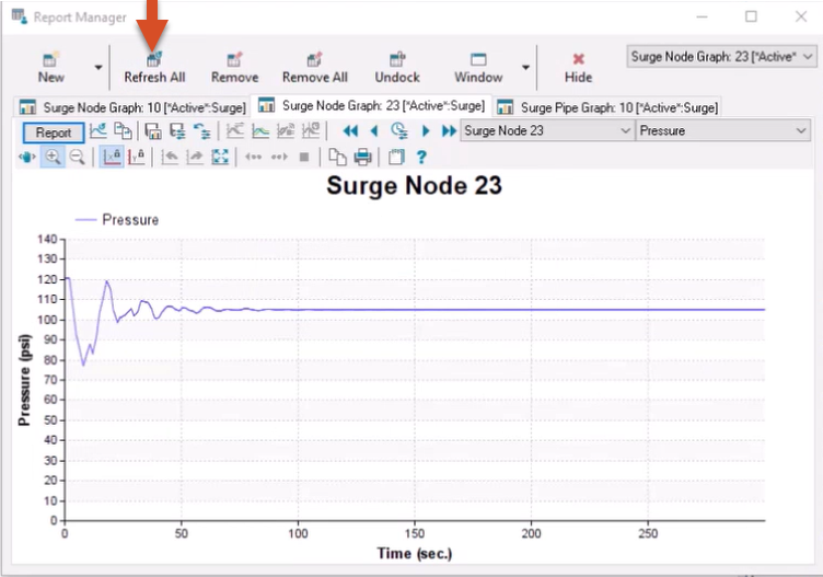
Then, open the Report Manager and refresh the output results to view them.
04:16
While there is still a transient event, allowing a slower rate of demand increase greatly reduced the pressure surge.
04:23
Close the Report Manager when you finish reviewing the results.