00:04
To best understand how InfoSurge Pro performs a surge analysis,
00:08
it is a good idea to experiment with a simple single-pipe model.
00:12
This can help you understand the various concepts and common procedures involved in running simulations and examining the results.
00:20
To begin, double-click the desired project .aprx file to open ArcGIS Pro.
00:26
Once the project starts, click the InfoWater Pro tab to open the InfoWater Pro ribbon.
00:32
In the Project panel, click Initialize.
00:36
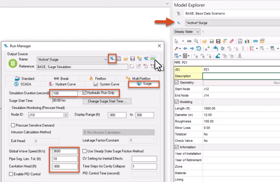
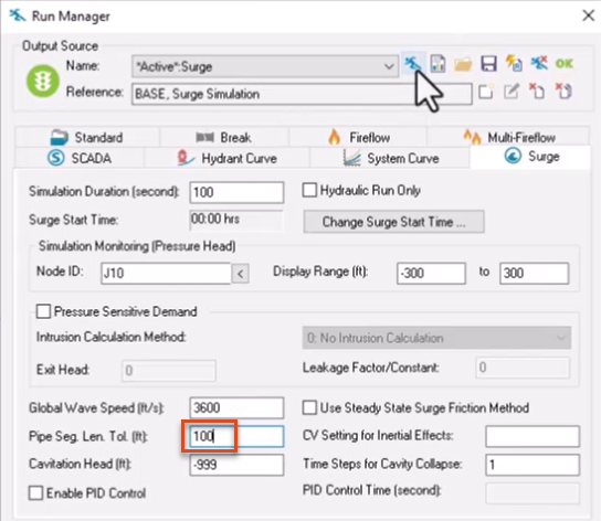
From the Model Explorer, click the Run Manager button to open the Run Manager dialog.
00:41
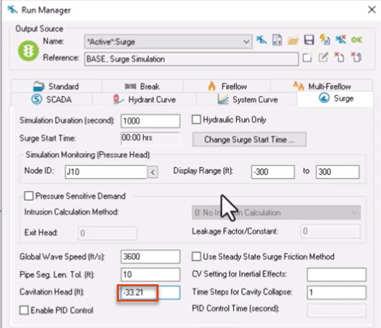
From the Surge tab: Set the Global Wave Speed to 3600 feet per second.
00:47
Set the Pipe Segment Length Tolerance to 10 feet.
00:52
Set the Cavitation Head to -999 feet.
00:56
Cavitation head is the head at which fluid will cavitate.
01:00
Note that this is a hypothetical value, as it is typically around -33 feet.
01:06
Set the Simulation Duration to 100 seconds.
01:09
Then, enable the Hydraulic Run Only option.
01:13
Click the Run button to run a hydraulic simulation, and then OK to close the Run Manager dialog.
01:20
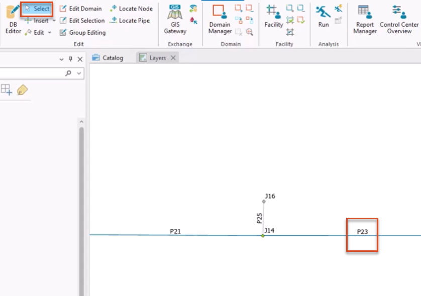
With the Select tool active, select the pipe with the ID P23.
01:26
In the Model Explorer, scroll down to view the hydraulic results for the steady state simulation.
01:32
Note that in this example, the Pipe Flow is 2663.98 gallons per minute,
01:39
with a Velocity of 7.56 feet per second.
01:43
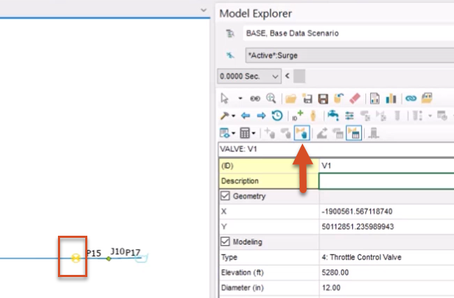
Now, from the map, select valve V1 to view its hydraulic results.
01:47
Note that the Upstream Hydraulic Pressure is 3.86 psi.
01:52
You can use these results to calculate the approximate surge pressure
01:57
immediately upstream of Valve V1 using the Joukowski equation.
02:01
This equation multiplies the change in velocity by the pipe wave speed.
02:06
This number is then divided by gravity and results in the change in hydraulic head,
02:10
which uses feet for its units.
02:13
The final calculation would be converting this head value to pressure by dividing by 2.31.
02:19
For this example, the simulation calculates results as a steady state, so you would use the velocity 7.56 feet per second.
02:29
The selected pipe does not have a wave speed, so the global wave speed of 3600 feet per second would be used.
02:36
To maintain the correct units for these calculations,
02:39
gravity would be 32.2 feet per second squared.
02:44
Using these numbers, the final calculation for the potential surge pressure would be 365 psi.
02:51
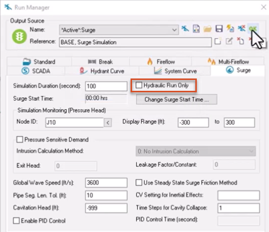
Valve V1 is a surge Active Valve (AV), assigned a stem change curve that closes the valve within ten seconds.
02:59
To view the upstream pressure profile of the valve, reopen the Run Manager dialog and uncheck the Hydraulic Run Only option.
03:06
Run another surge analysis, and then click OK when it completes.
03:12
From the ribbon, View panel, click Report Manager.
03:18
In the Report Manager dialog, click New.
03:22
Select *Active*:Surge as the Available Output Source.
03:26
From the Graph Report tab, pick Surge Pump/AV Graph, and then click Open.
03:32
Now, select valve V1 to view its upstream pressure profile.
03:37
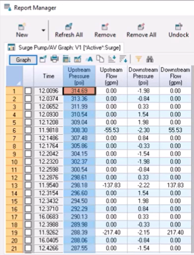
You can also click Report, right-click the Upstream Pressure (psi) header,
03:43
and then pick Sort Descending to bring the largest value to the top row.
03:48
In this example, the maximum surge pressure upstream peaks at 314.69 psi.
03:55
Click Hide to close the dialog.
03:57
Now, change the closure time of valve V1 to see how it impacts results.
04:04
Select valve V1 again, and then from the Model Explorer, click the AV (TCV) Operation Change button.
04:11
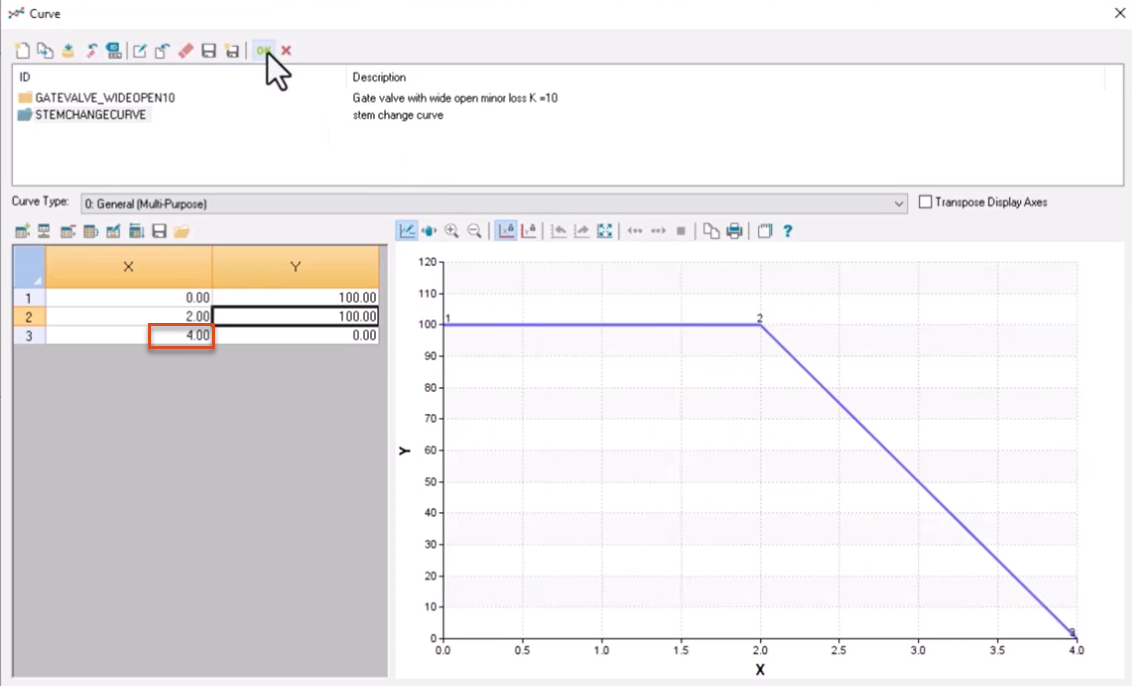
In the dialog that opens, next to the Stem Change Curve drop-down,
04:14
click the Browse button to open the Curve dialog.
04:18
With STEMCHANGECURVE selected, in the curve table, adjust the value in the third row of the X column to 4.
04:25
This changes the valve time from ten seconds to two seconds.
04:28
Click OK to save the changes and close the dialog.
04:33
In the AV (TCV) Operation Change Data dialog, click Update.
04:38
Now, open the Run Manager again, run another analysis, and then click OK when it is complete.
04:46
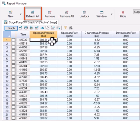
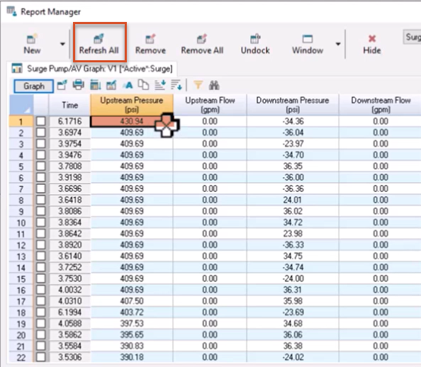
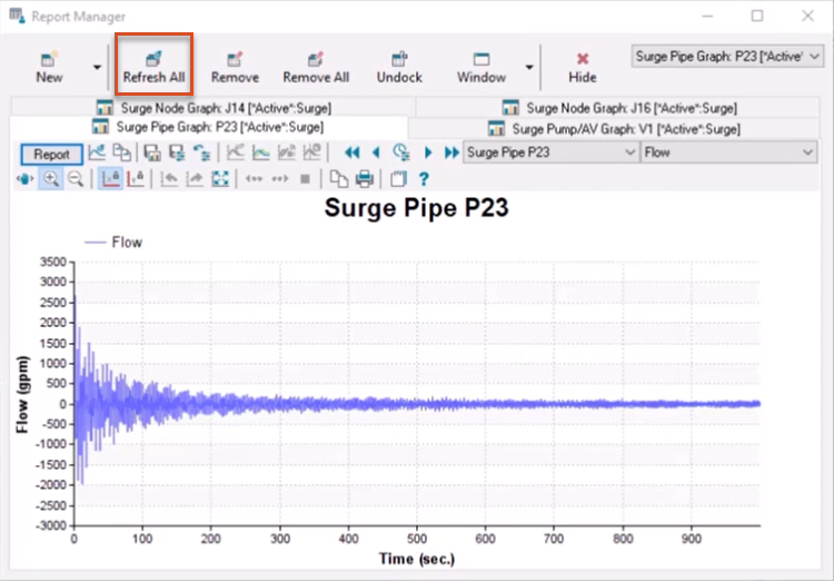
Reopen the Report Manager and click Refresh All to update the results.
04:51
Note that with the decrease in closure time, the maximum upstream pressure increased to 388.31 psi.
04:59
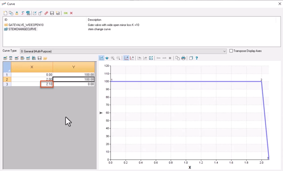
Repeat the process of changing the valve closure time, adjusting it to 2.10.
05:06
This changes the closure time from two seconds to 0.1 seconds.
05:12
Run another surge analysis and view the results in the Report Manager.
05:17
In this example, the maximum upstream pressure increased again to 430.94 psi.
05:25
Click Hide to close the dialog.
05:28
Try making various other changes to the network and perform additional runs to see how they impact results.
05:36
To simulate the effect of changing the pipe segment length tolerance:
05:40
For valve V1, in the Run Manager dialog, Surge tab, set the Pipe Segment Length Tolerance to 100 feet,
05:48
and then change it to 1 foot, performing two separate runs.
05:52
View the results in the Report Manager, noting the changes in maximum upstream pressure and the time each run takes to complete.
06:02
Generally, the larger the pipe segment length tolerance value, the longer the run takes to complete.
06:09
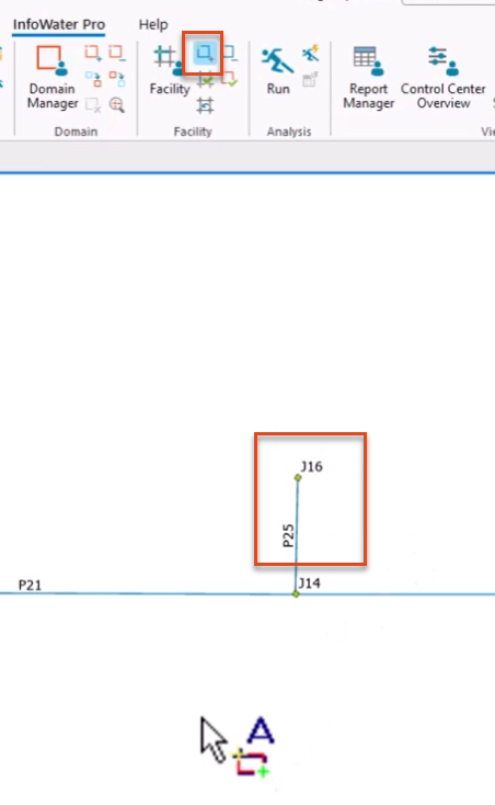
To simulate a dead end wave reflection: From the ribbon, Facility tab, click Activate Facility.
06:18
With the tool active, on the map, click and drag to select pipe P25 and junction J16.
06:26
From the Edit panel, enable the Select tool.
06:31
Reopen the Run Manager, change the Pipe Segment Length Tolerance to 100 feet, and then enable Hydraulic Run Only.
06:39
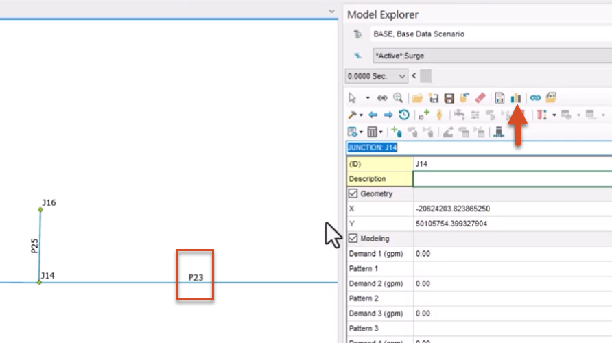
Perform another run, and then pick junctions J16 and J14 in turn to view their results in the Model Explorer.
06:49
Observe that both junctions have a static pressure of 23.59 psi.
06:57
Open the Run Manager once again, disable the Hydraulic Run Only option, and run the simulation one more time.
07:06
Close the Run Manager, and view the Report Manager results for J14 and J16,
07:13
noting their maximum pressures.
07:16
In this example, the pressure at J16 is higher than it is for J14.
07:20
Because J16 is a “dead end,” the transient wave is reflected here at twice the pressure head of the original wave.
07:28
To simulate how friction impacts pipe flow over time:
07:36
Then, from the Model Explorer, click Graph to view its flow profile.
07:41
Note that flow decreases as time progresses.
07:44
In the Run Manager, Surge tab, change the Simulation Duration to 1000 seconds.
07:52
Rerun the surge analysis, and then refresh the results in the Report Manager.
07:59
Note that by viewing results over a greater time,
08:03
you can observe that the pipe flow eventually approaches a steady state.
08:07
To simulate a cavitation event:
08:11
From the Run Manager, Surge tab, adjust the Cavitation Head to -33.21 feet.
08:18
Run another surge analysis and then, in the Report Manager, review the refreshed results for valve V1 .
08:27
Note that the surge pressure does not approach 0 over time.
08:32
This is because the cavitation head changed from -999 to -33.21 feet, the head at which cavitation typically occurs.