00:04
Water pro can test for chemical propagation
00:06
in a water quality modeling simulation.
00:09
The movement of water quality constituents is tracked
00:12
throughout the network during an extended period.
00:15
substances such as chlorine
00:17
total dissolved solids,
00:20
sodium fluoride and more can all be studied
00:24
in this exercise. You'll perform a chlorine analysis
00:28
to begin. Double click the desired project dot APR
00:35
Once the project starts,
00:36
click the info water pro tab to open the info water pro ribbon
00:41
in the project panel, click initialize
00:44
you start the chlorine analysis process by setting up the simulation options
00:49
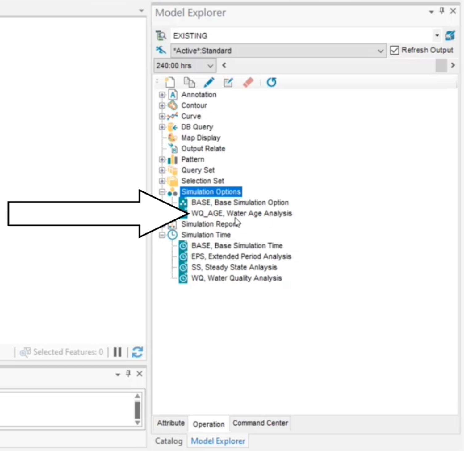
in the model explorer on the operation tab, expand the simulation options folder
00:54
and then double click W Q
00:56
age water age analysis
00:59
in the simulation options window on the toolbar, click the clone icon
01:05
in the new simulation options pop up. Enter a new id of W
01:09
Q underscore cl comma chlorine analysis
01:16
Switch to the quality tab,
01:19
select the chemical slash temp option
01:21
and then set the chemical name to chlorine.
01:26
Ensure the W Q tolerance is set to 0.1
01:30
and the mass unit is milligrams per liter
01:34
change the global bulk coefficient to negative one
01:38
and the global wall coefficient two negative 0.5
01:42
recall that bulk and wall coefficients represent
01:45
growth or decay rate for the constituent due
01:47
to reactions between the chemical and the bulk
01:50
flow of water or tink walls respectively.
01:53
Since both of these values are negative, these are decay rates.
01:59
Next, you need to set the chlorine concentration for the reservoir in the network.
02:04
In the map, select the reservoir W T P 100.
02:08
Then in the model explorer on the attribute tab
02:11
expand the tools drop down and select initial water quality
02:16
in the reservoir. Initial quality pop-up, enter a value of 1.2
02:20
and then click create
02:23
this represents a constant chlorine concentration of 1.2 mg per liter.
02:27
Leaving the treatment plant.
02:29
You are ready to run the simulation
02:32
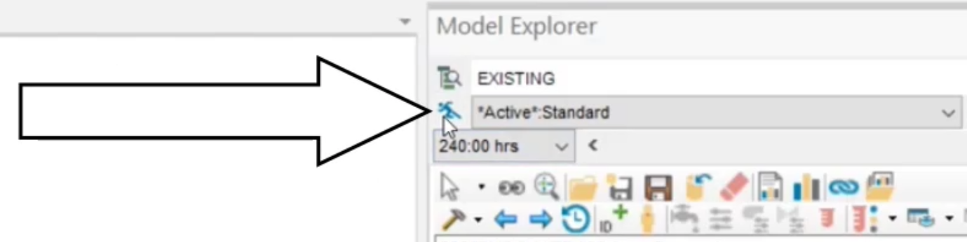
in the model explorer, click the run icon to open the run manager
02:36
in the standard tab. Expand the simulation options and select W
02:40
Q CL chlorine analysis.
02:43
Then expand the time setting and select W
02:46
Q water quality analysis.
02:49
Click the run icon and then click OK.
02:52
When the simulation has completed successfully
02:56
to view the results of your chlorine analysis simulation.
02:59
First select any junction in the map
03:02
in the model explorer on the attribute tab, click the graph icon
03:07
in the report manager that opens, change the graph parameter to chlorine.
03:12
Then from the toolbar, click new to create a new report
03:17
in the output report slash graph dialogue, click tabular report
03:21
and then select junction range
03:24
under data scope, select complete report slash graph and then click open
03:32
in the report manager for this tabular report,
03:34
expand the parameter dropdown list and select chlorine.
03:39
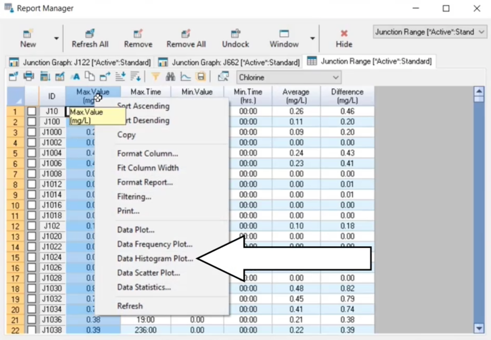
Then in the table, select the max value column header.
03:42
So the entire column is highlighted
03:45
right, click the max value column header and select data histogram plot
03:50
in the data histogram of max value dialogue, select by interval,
03:55
enter a value of 0.5
03:58
and then click classify
04:03
Now details the chlorine residual distribution in the
04:06
system using 0.5 mg per liter classes.
04:10
When you are finished reviewing the report,
04:12
close the histogram and then click hide to close the report manager.