00:04
WS pro the drain down and recharge simulation
00:08
options in the run schedule can improve the
00:10
model accuracy for a situation in which a
00:12
network loses pressure and pressure is later recharged.
00:17
This simulation can highlight the locations of the first and last customers
00:22
to lose pressure and how long it could take to regain it
00:26
in this exercise. Part of a small network is isolated for a water quality issue
00:32
in the model group window under the drain down model group click and
00:36
drag the drain town network into the workspace to open the GEO plan.
00:41
This small network is supplied by a simple fixed
00:44
head node representing a pumping station to the east
00:47
to simulate drain down.
00:49
You will close an isolation valve just downstream of
00:51
the pumping station to see the effect on the network
00:55
first. Create a new scenario by clicking the create scenario button in the toolbar.
01:01
In the new scenario, name field type in the name isolation,
01:07
Then zoom into the area of the
01:09
network immediately downstream of the pumping station.
01:13
Double click the valve in the upper part of the T
01:15
junction with the asset ID 205301 to open its properties.
01:22
Scroll down in the valve object properties window and under valve control,
01:26
find the mode id field.
01:29
It is currently set as a TV,
01:31
a throttled valve which does not change during a simulation.
01:35
You need to change it to a time controlled valve T CV.
01:39
So you can open and close it during the simulation to model a temporary shutdown,
01:44
expand the dropdown and select T CV.
01:48
You now have the option to edit the profiles field.
01:52
Click the more button with the ellipsis to open a dialogue where
01:55
you can edit the date and time of the valve opening and closing
02:00
In the date and time column,
02:02
either expand the drop down to set the
02:04
following dates and times or type them in manually
02:08
in the first row. March 1st 2023 at midnight
02:13
in the second row, March 1st 2023 at six AM
02:18
and in the third row, March 1st 2023 at seven PM
02:24
in the opening percentage column type in the following values
02:28
in the first row, 100
02:31
in the second row zero
02:33
and in the third row 100
02:36
this means the valve is set to be fully open at midnight,
02:40
close at six AM, then open again at seven PM.
02:47
In the toolbar, click save data to commit the changes you just made to the database.
02:52
Click OK? In both notifications that follow
02:56
then, right click the drain down model group and create a new run group and run
03:04
in the schedule. Hydraulic run dialogue in the title field.
03:07
Enter the name isolation base.
03:10
Enable the experimental option
03:13
with the required items.
03:14
Tab open click and drag the drain town network to the network pa in the dialogue.
03:21
the control and demand diagram pans populate automatically because
03:25
they were previously associated with the drain town network.
03:29
Next, open the scenarios, tab
03:32
disable the base option and then enable isolation,
03:36
click save and then run
03:40
info works. WS pro does not simulate draind down by default.
03:43
So the results of this run will serve as a before snapshot for comparison later,
03:50
once the run is finished, click and drag the results to open them in the GEO plan
03:55
in the tools, toolbar,
03:56
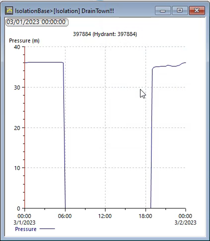
click the graph tool and then click any hydrant downstream of the valve.
04:01
In this example, a hydrant with the asset ID 397 884 is selected.
04:08
The graph indicates a total loss in pressure at six AM when
04:12
the valve closes and pressure then returns to normal at seven PM.
04:16
After the valve opens again,
04:19
you can also select any link to view similar effects on flow.
04:25
you have the option to run a query to find
04:27
out how many customers were isolated during this operation.
04:31
Expand the stored query group, then click and drag.
04:34
Select isolated customers to the GEO plan to run it.
04:39
This automatically selects all customers in the network
04:41
who were isolated for longer than one hour.
04:45
every customer highlighted in red downstream of the valve is affected.
04:50
Now run the isolated customer count query.
04:53
A small grid appears in the workspace indicating
04:56
that 230 customers were isolated during the operation
05:01
in the replay toolbar. Click clear results.
05:05
Now you'll run another simulation this time with draind down enabled
05:10
double click the isolation base run to open the schedule,
05:13
hydraulic run dialogue again,
05:15
change the name to isolation, draind down and then click save.
05:21
Note that the new run displays in the model group window
05:25
in the run parameters group box,
05:27
expand the dropdown and select simulation options.
05:31
Then click the options button
05:33
in the simulation options window enable allow drain down and allow recharge,
05:40
close the window. Then click save and run in the dialogue.
05:45
Open the results by clicking and dragging them to the GEO plan
05:50
with the graph tool enabled. Click the same hydrant as you did. After the base run,
05:56
the graph shows that instead of the pressure dropping to zero,
05:59
it stops at a lower value and then gradually decreases until around six PM.
06:04
Repeat this action by graphing any link downstream
06:07
from the valve to see that flow is also
06:09
impacted during the isolation period but is not immediately
06:12
interrupted as it was in the base run.
06:16
run the select isolated customers and isolated customer count queries.
06:21
The select isolated customers query shows far fewer customers are isolated
06:26
for longer than one hour than in the base run.
06:28
Customers not highlighted retain water pressure,
06:31
albeit lower pressure rather than losing it completely.
06:35
The isolated customer count query shows far fewer customers. Only 60.
06:39
In this case are isolated.
06:42
You can also visualize the run results using a long section
06:47
toolbar enable the trace and select links upstream tool and then find
06:52
the southwestern most point in the network and click to highlight it.
06:56
This runs a trace back to the water source.
06:60
Now from the windows toolbar,
07:02
click the new long section tool to view the
07:04
traced portion of the network as a long section,
07:08
click the long section window and select
07:10
properties to open the section properties dialogue
07:13
for better visual clarity.
07:15
When viewing the long section disable the option to show min
07:23
In the long section window,
07:25
the horizontal blue line indicates the pressure level in
07:28
relation to the position within the long section.
07:32
In the replay toolbar,
07:33
click play to step through the simulation
07:35
timeline and observe how the pressure changes at
07:38
six AM when the valve is closed and then gradually decreases until seven PM.
07:44
Portions of the network immediately downstream of
07:46
the isolation lose pressure during this time.
07:49
But areas further downstream, maintain pressure
07:53
at seven PM. The isolation valve reopens and the network is recharged.