00:04
Once you have established a connection between live data and a network,
00:07
you can use the data to perform a run and graph
00:10
the results to see how the system performed in real time.
00:14
First create a new run with the live data connected to the network.
00:18
You can create a new run or use an existing one.
00:22
In this example, Bridgetown base already exists in the run group,
00:27
double click to open it.
00:28
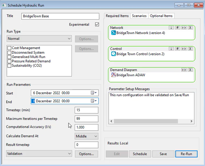
And in the schedule, hydraulic run dialogue,
00:30
update the network and control to the latest versions
00:35
in the run parameters group box change the start to 6th December 2022 by
00:40
clicking on each section of the field and typing the day and month.
00:45
Then adjust the end to 8th December 2022.
00:49
Note that these dates match those in the live data files connected to the network.
00:54
Click save and then rerun,
00:58
open the results by clicking and dragging the bridge con run onto the GEO plan.
01:04
Then with the graph tool selected,
01:06
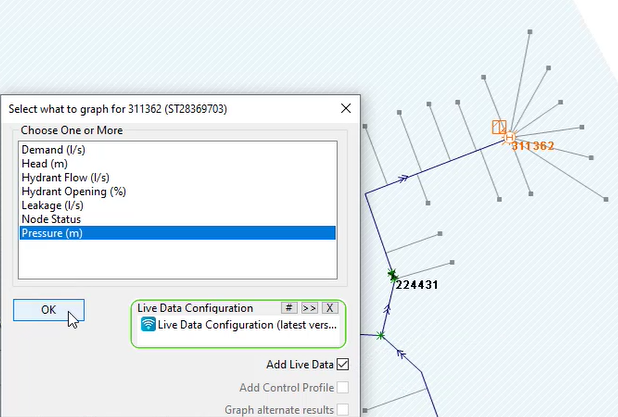
select a network object with live data attached to it.
01:11
In this example, hydrant 311 362 is selected
01:15
with the select what to graph four dialog,
01:17
open click and drag the live data configuration
01:20
to the live data configuration group box.
01:24
Select pressure meters, check the box next to add live data, then click OK.
01:30
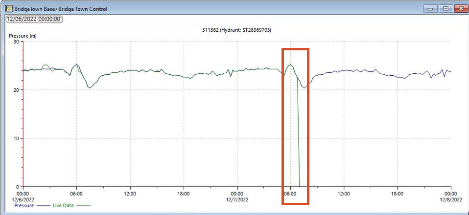
A graph opens showing the pressure as a blue line and the live data as a green line
01:36
note that there was a pressure drop in the live data around seven AM.
01:41
If the time you run the model for exceeds the time of the live data,
01:44
the live data would simply stop at that point.
01:47
However, in this example, the live data shows the pressure dropping to zero.
01:53
That means that somewhere in the live data files or through your telemetry system,
01:57
something has happened in the network to cause a drop in pressure.
02:01
For example, a burst pipe or telemetry system drop-off may have occurred,
02:06
you can graph other objects with the available live data to see similar results
02:10
that also show the rapid drop in pressure occurring at around seven AM.