00:03
works W S pro allows you to model pumps and pump curves,
00:07
pumps are widely used in water supply systems.
00:11
Pumps operate on a pump curve which contain
00:13
operating characteristics like head and power consumed.
00:17
The pump curve provides a relationship between the flow head and electric
00:22
power to determine the nominal actual and minimum maximum speed curves,
00:27
power curves and efficiency curves.
00:32
you will be working in a small network modeled with a fixed head
00:35
supply to the east representing a reservoir with a top water level tw
00:42
L of the reservoir does not provide enough pressure alone to supply the network.
00:47
So you must determine how much pressure is needed to address the problem.
00:52
First, open a new transportable database
00:56
from the file tab click open open transportable database.
01:00
Navigate to and open the file identifying pump requirements dot WPT
01:06
from the transportable database window,
01:08
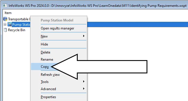
right, click pump station and select copy
01:13
in the model group window,
01:14
right? Click the database and select paste pump station with Children
01:21
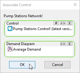
right? Click the pump stations network and select associate control,
01:26
click and drag the control and demand diagram.
01:29
Pump stations control and pump stations average demand to
01:32
their respective areas in the associate control dialogue.
01:37
Click ok. And then open the pump stations network.
01:43
First you will run the model to see what the results are.
01:47
Right. Click the pumps model group and select new run group.
01:52
Click ok. To accept the default name
01:56
right click the run group and select new run
02:01
in the schedule. Hydraulic run dialogue in the title field type in base
02:06
click and drag the Newtown network to the network area in the dialogue,
02:14
Then in the model group window,
02:16
click and drag then results into the GEO plan to open them
02:22
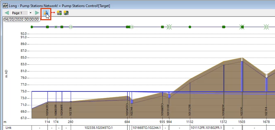
zoom into the far right area of the network.
02:26
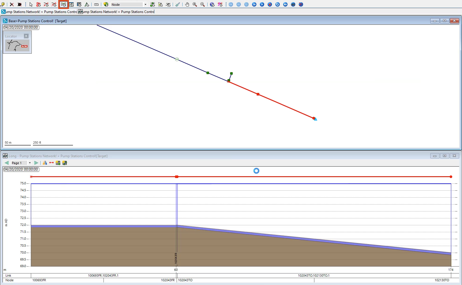
Click the link immediately downstream from the fixed head,
02:29
which is represented by a blue triangle icon to select it.
02:34
Then in the toolbar, click the long section pick button
02:38
with the tool active, click the next link downstream.
02:42
As soon as you do, the long section appears below the model.
02:46
This tool continues to trace along the network
02:48
in that direction until it reaches a junction,
02:52
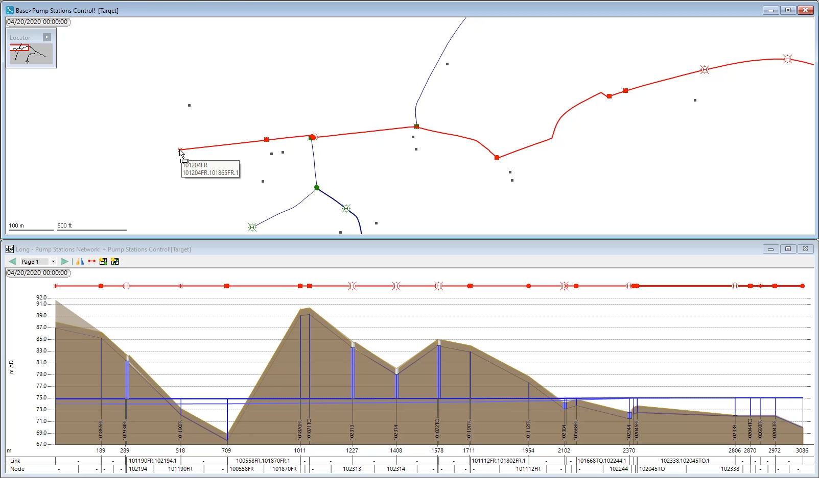
continue to trace the links as seen in this example. Until you reach node 101204. Fr
02:60
you can see that as you click each node, the long section continues to be built
03:04
to avoid having to manually retrace this long section.
03:07
You can create a new selection list by right clicking selection list group.
03:11
In the model group window and picking new selection list,
03:16
choose a name for it and then click ok.
03:20
Alternatively, after tracing the desired section,
03:23
you can click the new long section button in the toolbar
03:26
in the toolbar, click the select tool to reactivate it.
03:30
Click somewhere in the GEO plan to deselect the long section
03:35
in the long section window.
03:37
Observe how the hydraulic profile of the section reads from right to left with the
03:41
fixed head on the right and the end of the section on the left,
03:46
if you prefer the long section window to
03:48
display the hydraulic profile from left to right,
03:50
click the flip view button.
03:54
There are many display options for the long section window.
03:58
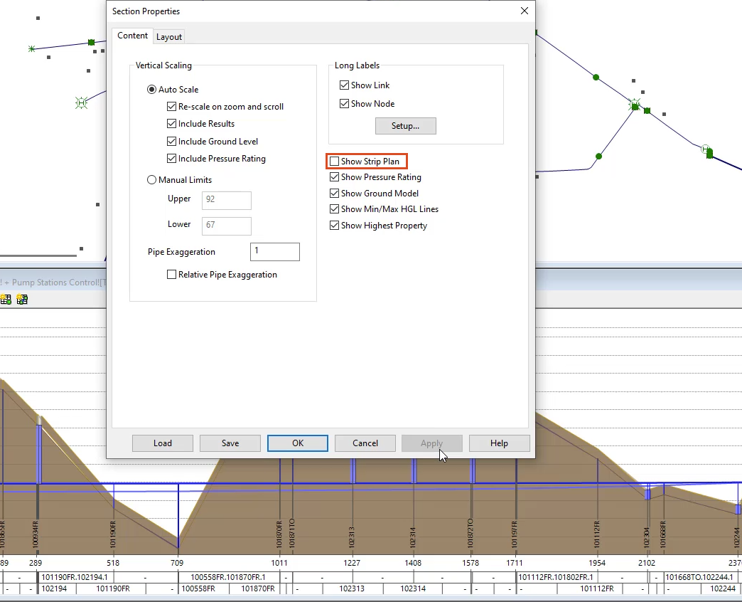
Right? Click in an empty part of the window and select properties
04:02
in the section properties. Dialogue. There are two tabs content and layout.
04:07
There are several customizable fields here including scaling
04:12
typeface and colors which you can use to change what is shown in the long view.
04:19
the strip plan is the line with icons representing
04:22
the different objects and nodes along the section path
04:25
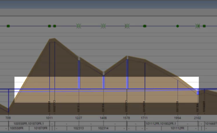
in the content tab deselect the checkbox next to show strip plan and then click apply
04:31
and observe how the strip plan disappears from the top of the long section window,
04:36
click the check box again
04:38
and then click apply to turn the strip plan back on.
04:42
You can use the graph tool and click those icons to graph the results
04:47
in the long section window.
04:48
You can see that the blue hydraulic grade line is
04:51
showing that there is insufficient water supply in the network.
04:55
This is represented by areas where the grade line is below the ground level.
04:60
With this information,
05:01
you can start to design a pump curve
05:03
and determine the characteristics of your pump station.