00:03
When performing a Multi Solute Water Quality simulation, after the MSQ model has been set up using the Solute Data Object dialog,
00:12
and after the network has been dosed with the contaminants, you can configure and run the MSQ simulation.
00:19
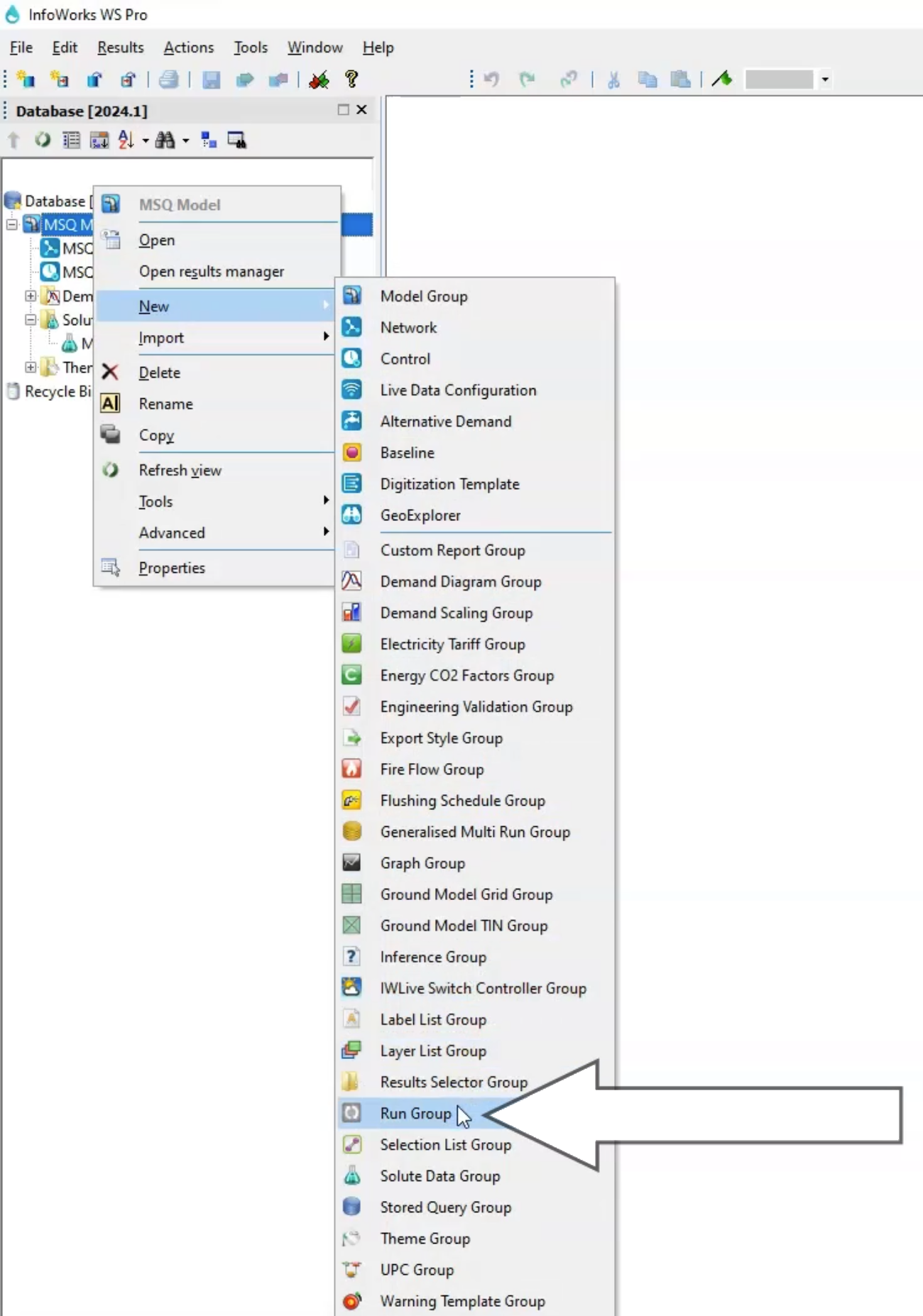
To start, create a new run group.
00:22
From the Model Group, right-click the MSQ Model and select New > Run Group.
00:29
In the popup, name it “Run Group” and then click OK.
00:33
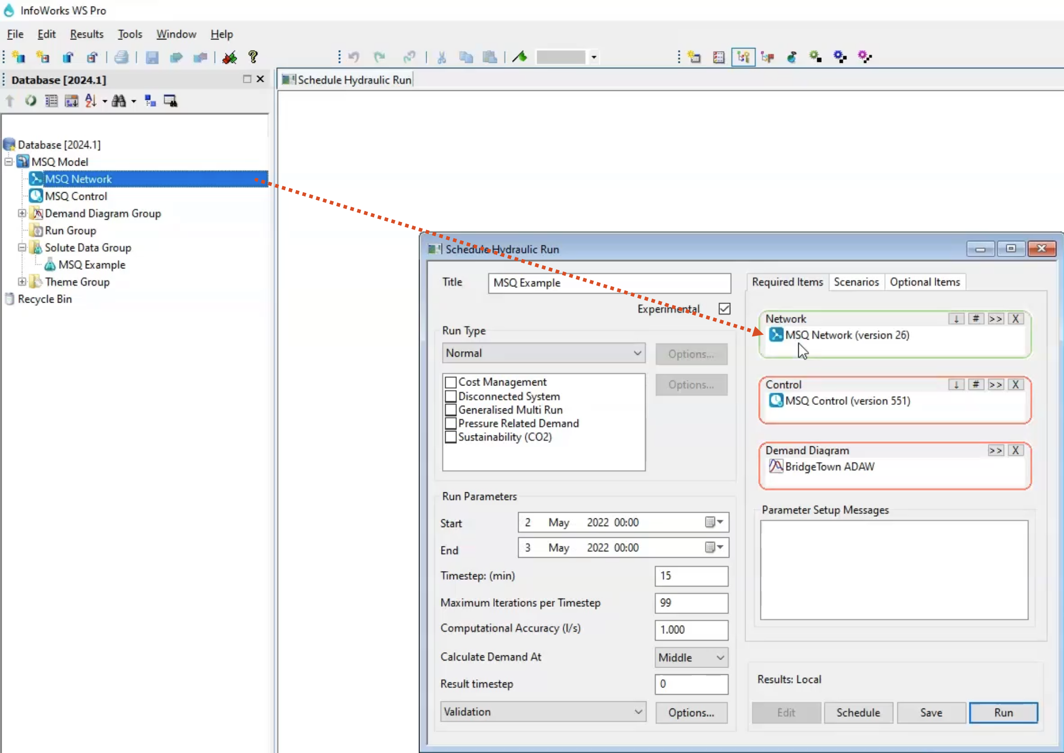
Then right-click the Run Group and select New > Run.
00:38
In the Schedule Hydraulic Run dialog box, name simulation “MSQ Example”, which is the same name as the new solute data.
00:46
Also enable the Experimental option.
00:50
Then, from the Model Group, drag and drop the MSQ Network, Control, and Demand Diagram into their respective boxes.
00:58
Set the run time to go from May 2nd, 2022 at 00:00 until May 4th, 2022 at 00:00.
01:06
In the Run Type group box, expand the drop-down and pick Water Quality.
01:11
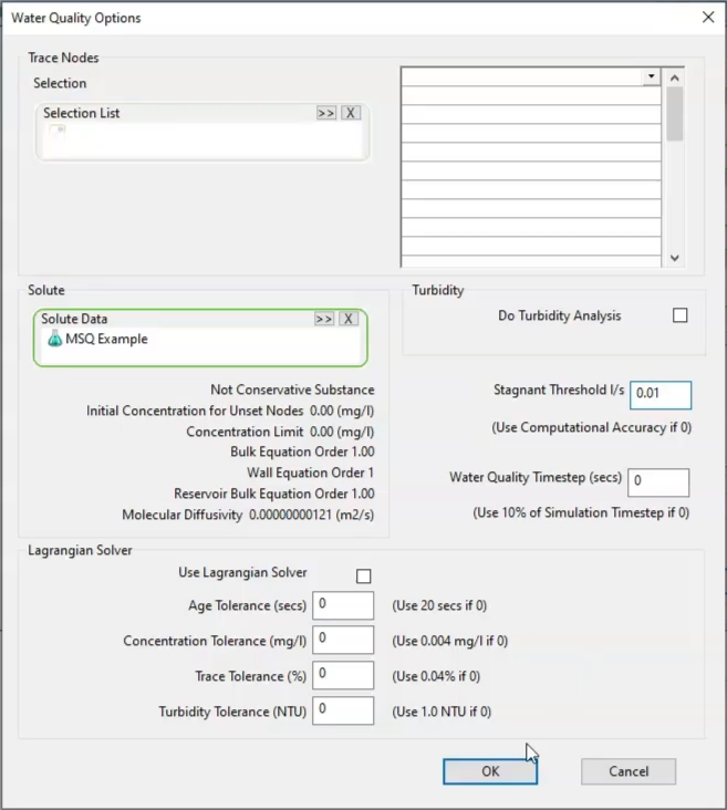
With the Water Quality Options dialog open, click and drag the MSQ Example solute data into the Solute group box.
01:19
Set the stagnant threshold to 0.01 l/s.
01:25
The stagnant threshold is the computational accuracy for water quality calculations.
01:31
If you leave it set to zero, it will use the computational accuracy of the hydraulic simulation.
01:37
Note that, if you close the Water Quality Options dialog,
01:41
you can easily reopen it by clicking the Options button in the Run Type group box.
01:48
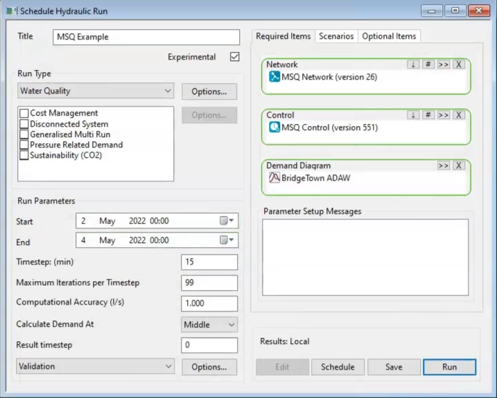
Back in the Schedule Hydraulic Run dialog, click Save and then Run.
01:54
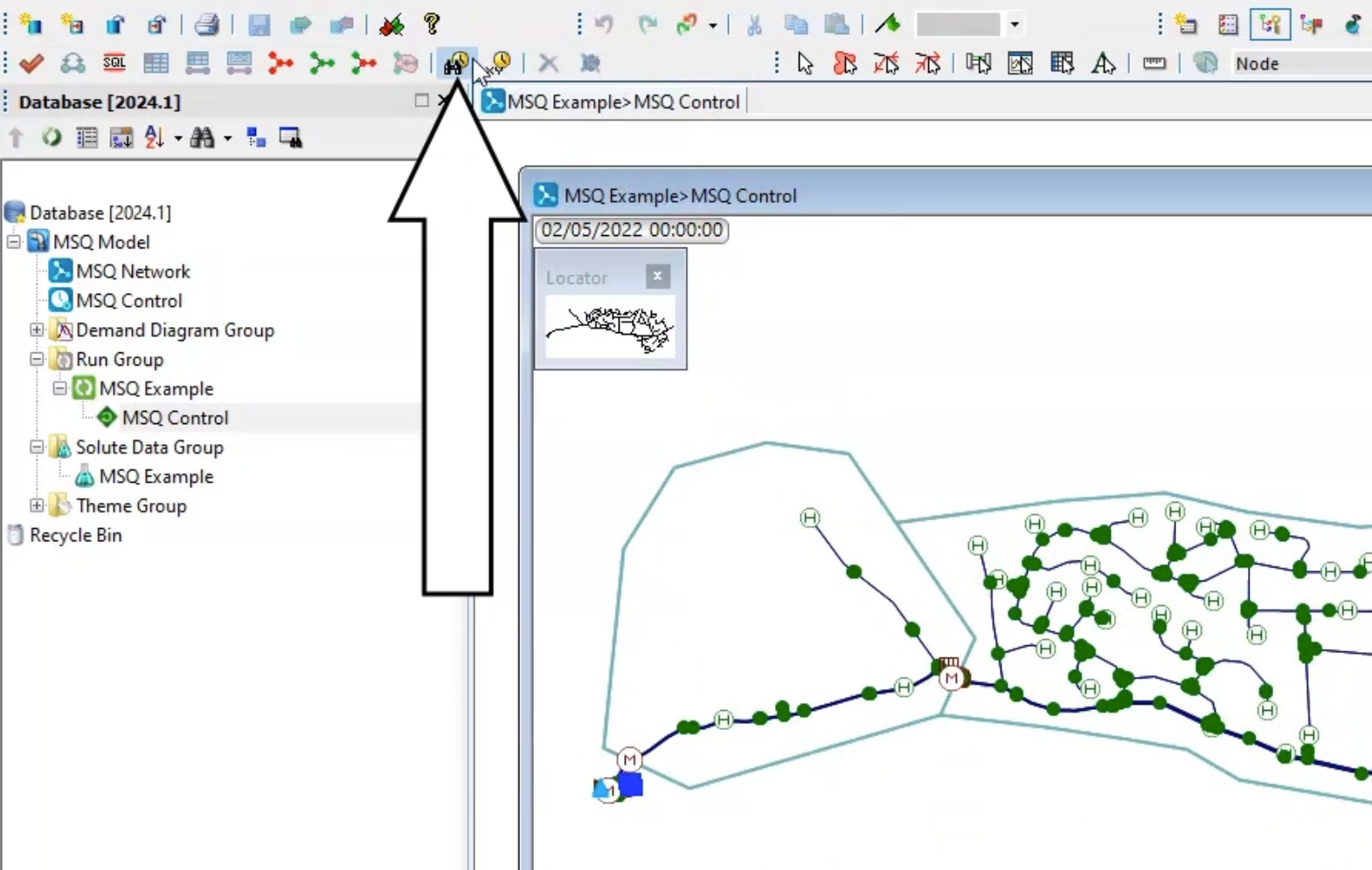
In the Model Group, the simulation results now appear under the MSQ Example run.
02:00
Click and drag the results to the GeoPlan.
02:04
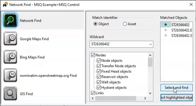
In the Tools toolbar, click the Find Network Objects tool.
02:08
In the Wildcard text box enter the NodeID ST26366402.
02:19
Close the Network Find window.
02:23
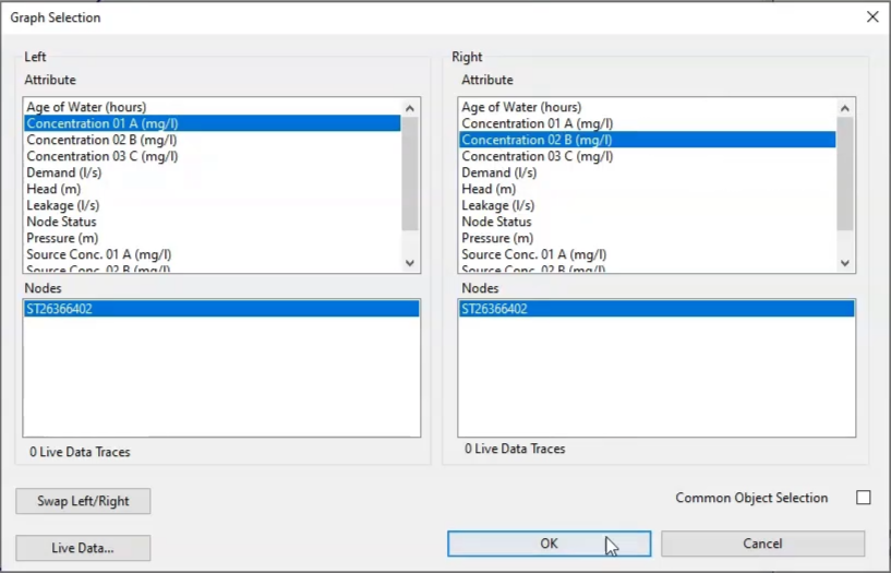
Then, click the Graph Selected Objects tool.
02:28
In the Graph Selection dialog, in the Left Group Box, select Concentration 01 A, and then in the Right Group Box, select Concentration 02 B.
02:41
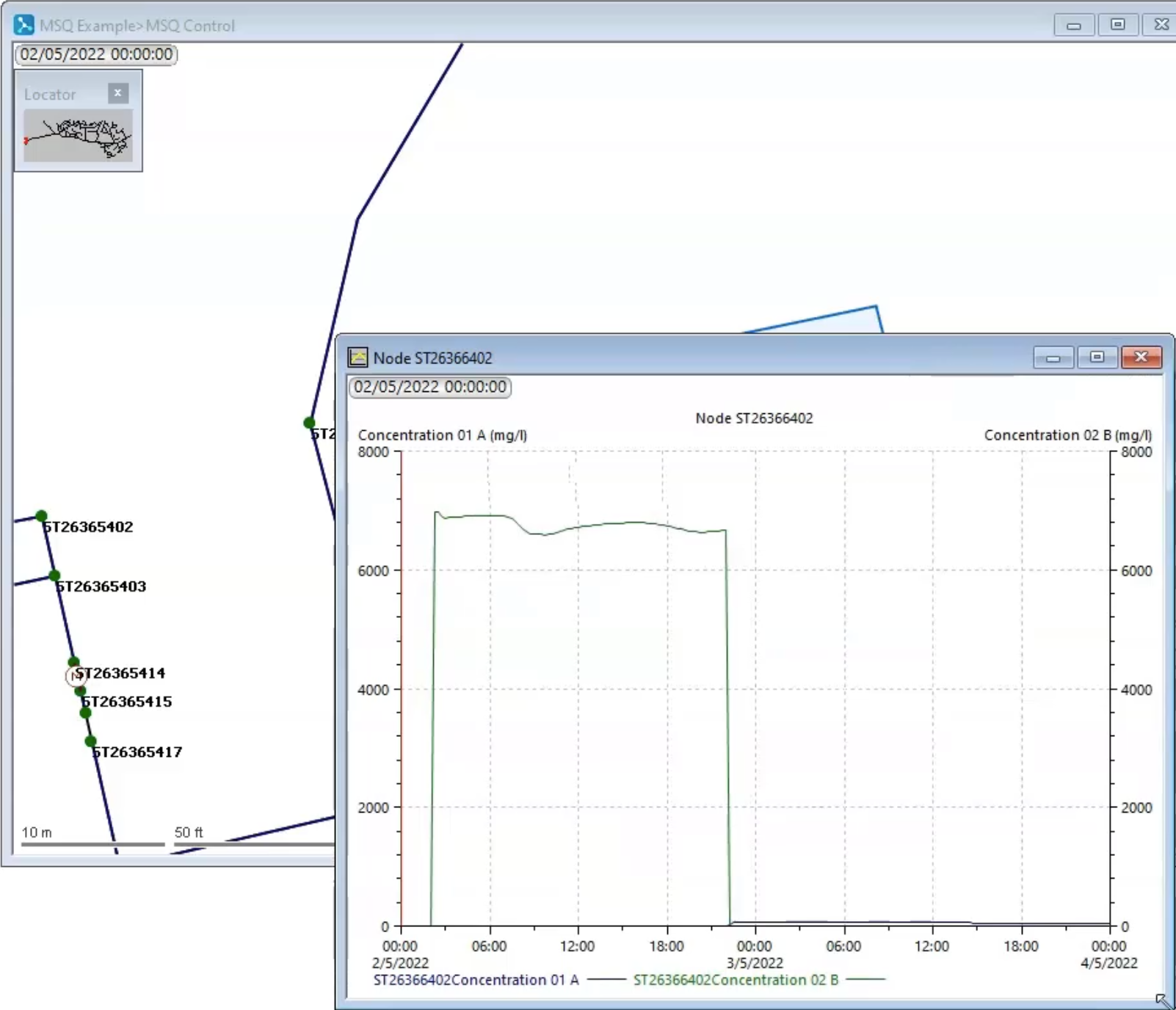
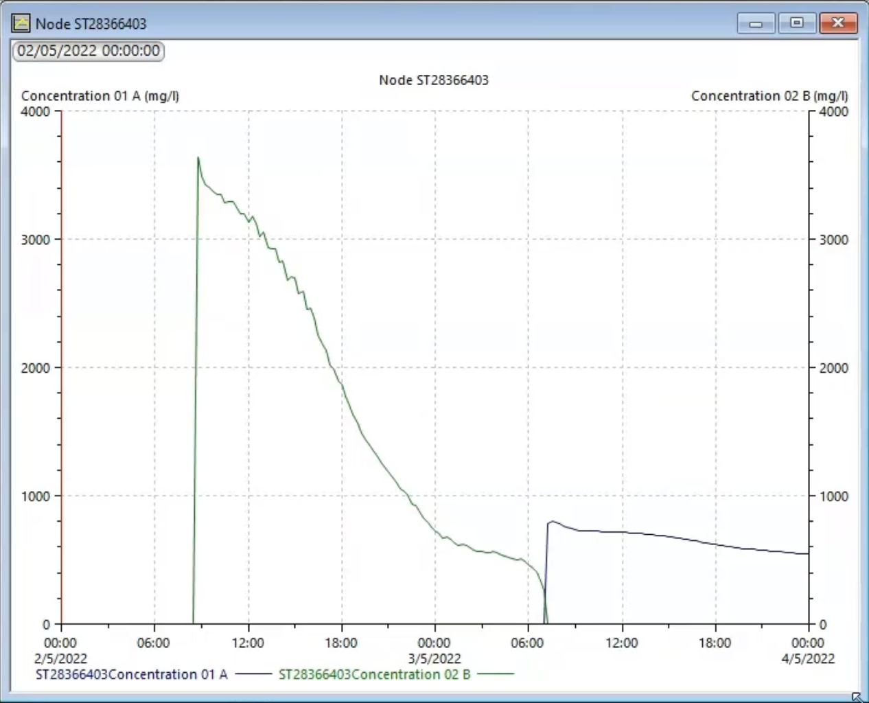
On the graph, you can see the concentration of the two contaminants at the point below the reservoir across the simulation.
02:48
Repeat this process for Node ST28366403.
02:55
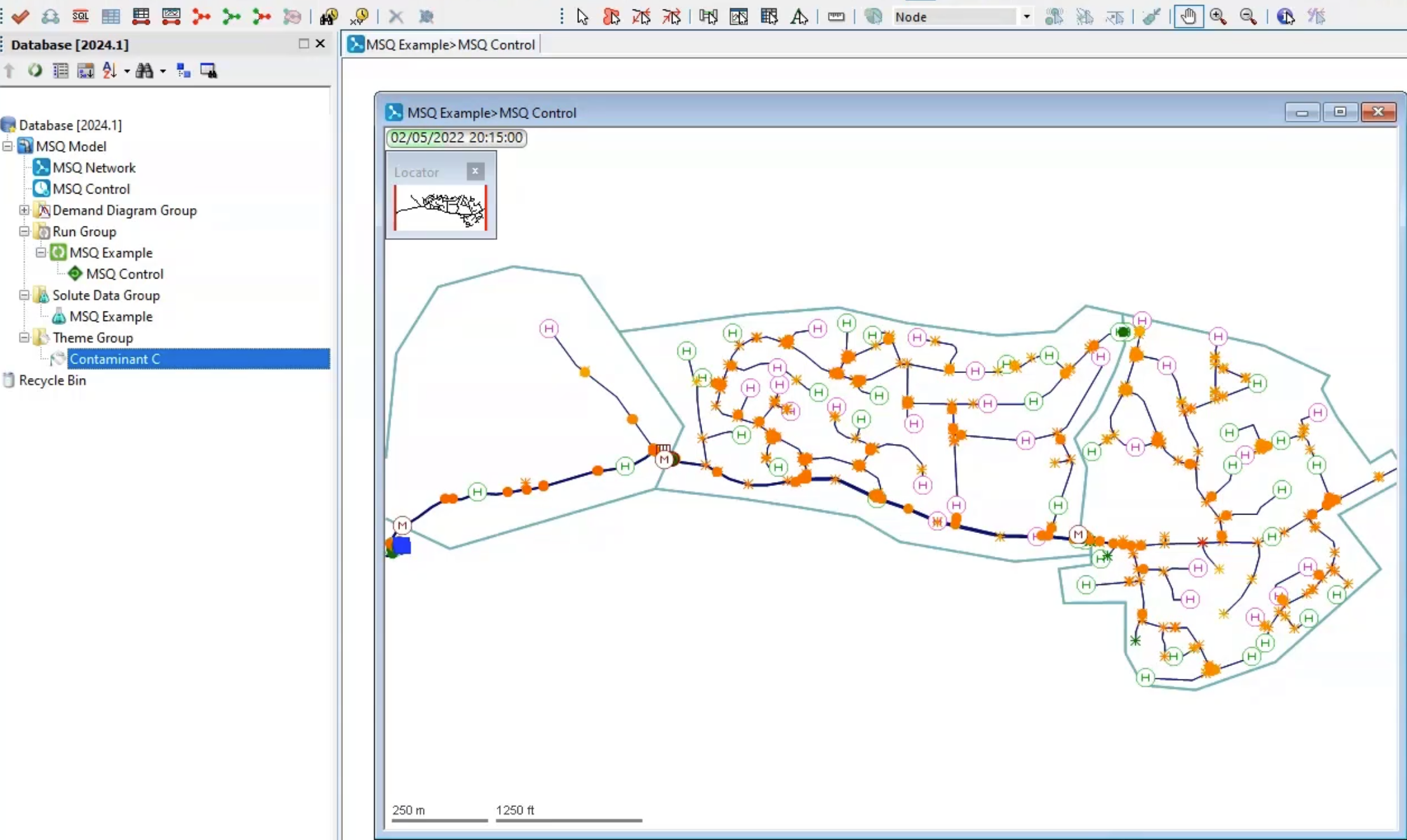
To see how Contaminant A and B react to form Contaminant C across the network,
02:60
double-click the Contaminant C theme
03:02
and play through the simulation to visualize the movement of Contaminant C through the network over time.