00:03
A prerequisite for network model calibration is that overall flow balances—
00:08
—demands, leakage, and transfers—
00:12
—are in reasonable agreement for both the model and the real-world network for the specified time period.
00:19
To determine the performance of the current network,
00:21
and to validate that a calibration exercise needs to take place,
00:26
you need to compare the simulated pressure and flows with observed values.
00:31
The simulated values are from the results of a normal hydraulic simulation,
00:36
and the observed values are provided by a live data configuration.
00:41
You can then compare the live and predicted results using either graphs or grid reports.
00:48
Observed vs Predicted Reports allow you to compare summary flow, pressure,
00:54
or reservoir depth for all network objects of an appropriate type in the model that are linked to live data.
01:01
Simulation Graphs allow you to produce graphs of the comparison between observed
01:06
and predicted data for all the selected objects of appropriate type that are linked to live data.
01:12
For this exercise, you will produce an observed versus predicted report.
01:17
Begin by running a normal hydraulic simulation.
01:21
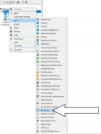
Create a new Run Group object.
01:23
In the Model Group, right-click the Calibration Model model group and select New > Run Group.
01:32
Then, right-click the new run group and select New > Run from the flyout.
01:39
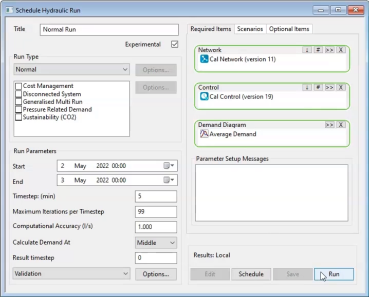
The Schedule Hydraulic Run dialog opens.
01:43
In the Title field, type a name for the run.
01:46
In this example, “Normal Run” is entered.
01:50
Check the box next to Experimental.
01:53
Then, from the Model Group, drag and drop the Calibration network into the Network panel in the dialog.
02:01
The Control and Demand Diagram panels populate as well.
02:05
Click Save, and then Run.
02:08
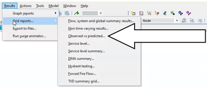
Next, to produce the observed versus simulated grid,
02:12
double click on the Cal Control simulation results, then expand the Results menu and select Grid reports,
02:21
and then from the flyout, select Observed vs predicted.
02:26
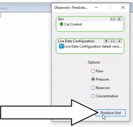
The Grid Report (Observed vs Predicted) dialog box appears.
02:31
From the Model Group, drag and drop the Normal Run simulation into the Sim panel,
02:38
and then drag and drop the live data configuration into the Live Data Configuration panel.
02:45
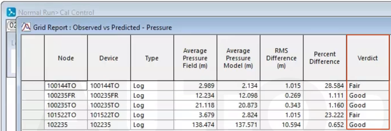
Under Options, enable Pressure, and then click Produce Grid.
02:51
A table appears, providing some values and a verdict for each point in the network that has a live data pressure feed associated with it.
03:00
In this example, you can see that three points have a fair verdict;
03:05
therefore, running the automatic calibration module may improve the performance.