Welcome back to our SPICE Simulation Series, Part 3! In Part 2 we showed you how to run a fundamental operating point analysis to simulate current and voltage at a single reference point. Now it’s time to ramp up the difficulty with DC sweep and AC sweep analysis. These two SPICE simulation methods sweep a circuit over a defined voltage or frequency range. This can give you an accurate representation of how your circuit will behave. Running these two simulations will also give us our first look at plot data, probes, multipliers, and more. Let’s get started!

DC Sweep Simulation

We’ll be using DC sweep to calculate our circuit’s bias point over a range of voltage values. By defining the start and stop voltage values we can get an accurate representation of how voltage fluctuates in specific scenarios.

Example Project

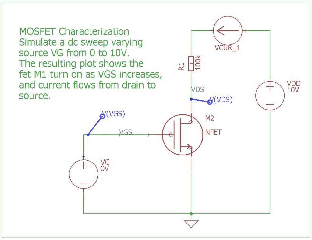
The example project we’ll be working with is a FET characterization schematic. Let’s open this now. Look for the Fet_Characterization project folder within the Projects » ngspice directory in your Autodesk EAGLE Control Panel. Then open FETCHAR.sch.

This schematic is a basic circuit that many beginner engineers use to learn what a FET is and what voltage curves look like in a SPICE simulation. With this circuit, we’ll be sweeping voltage from the FET gate to ground with a defined range of 0 to 10 volts.

Simulation Configuration

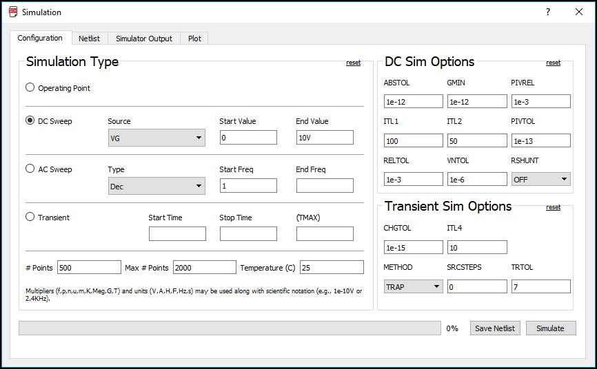
We’ll begin by selecting the Simulation  icon to open the Simulation dialog. Here we can see that DC sweep is the chosen simulation type with preconfigured Source, Start Value, and End Value parameters.

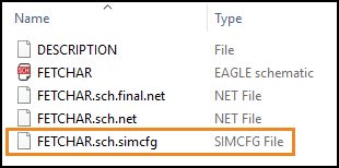
One important thing to note is that all of these values come up as presets because there’s a SPICE simulation file saved in this project’s folder. Every time you open the Configuration tab in a SPICE simulation and adjust settings, EAGLE saves a .simcfg file that sits next to your .sch file.

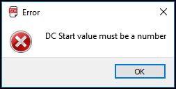
Before running our simulation, let’s talk about two quick points – range accuracy and multipliers. EAGLE always checks for proper parameters in your selected simulation type before the simulation completes. This might seem obvious, but it’s good to point out that the simulation simply won’t run if you enter an invalid start or end value. For example, if we were to enter a letter for the start value we’d get an error after selecting the Simulate button as shown below:

Next, take a look at the bottom portion of the Simulation dialog, and you’ll see a text description about Multipliers. This is explaining that you can use standard units in combination with scientific notification and multipliers to define specific frequency ranges or start values.

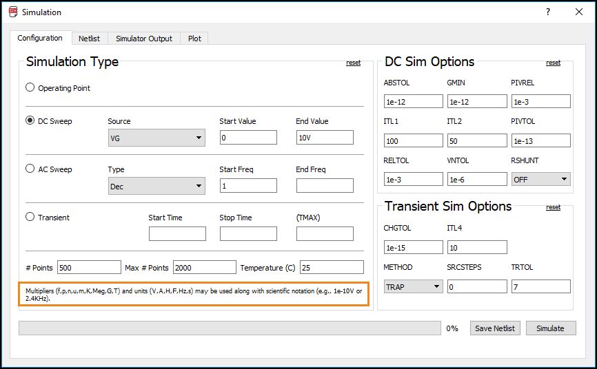
For example, if you were doing a transient analysis you could type in 1ms for the start time. For a stop time, you could use scientific notation and type in 5e-3s. Both methods of notation end up being translated in the same way, so it comes down to personal preference.

Simulation Analysis

Now that we have all the basics covered let’s run our DC sweep simulation. We’re going to sweep our gate voltage and should see the current increase as the transistor turns on. Press the Simulate button to see what happens.

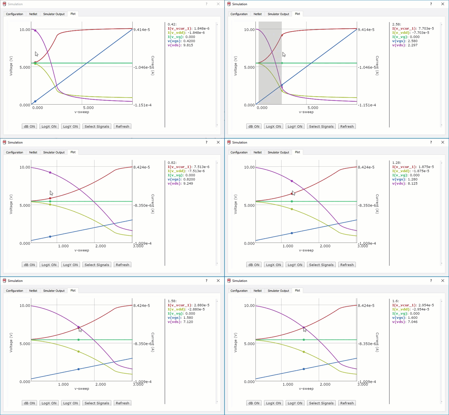
Notice that because we ran a DC sweep the results go directly to the Plot tab instead of the Simulator Output. Here we can see voltages on the left-side Y axis, current on the right-side Y-axis, and our voltage sweep range on the X-axis. vgs is what was swept.

If you move your cursor from left to right on the plot graph, it will follow all of the lines and update the values on the right-hand side. In this example, we want to determine the exact point where vds and vcur_1 intersect.

You can zoom into a specific point on the graph by left-clicking and drag over a specific area. Double-clicking will restore the default view. Here we can see that the FET turns on as vgs increases to about 1.6 volts. This is also the point where our current starts flowing from drain to source.

Great! Let’s move on to a more advanced simulation with AC sweep.

AC Sweep Simulation

AC sweep simulation is used when you want to calculate the small-signal response of a circuit. This method will first use operating point analysis to gather linear, small-signal models for all nonlinear components. The snapshot of this circuit is then analyzed based on a defined frequency range.

Example Project

The example project we’ll be working with is an RC filter schematic. Let’s open this now. Look for the rcfilter project folder within the Projects » ngspice directory in your Autodesk EAGLE Control Panel. Then open rcfilter.sch.

In this circuit we see the input signal, V1, flowing through three RC filters with different cutoff points. We’re expecting cutoffs to occur at 1.59KHz, 159KHz, and 15.9MHz. All of the resistor values are the same, so our focus will be on tweaking the capacitor values.

Simulation Configuration

We’ll begin by selecting the Simulation  icon at the top of our interface to open the Simulation dialog. Notice that AC sweep is already set up with some default values. Starting Freq is set to 1Hz, End Freq is set to 500 MHz. Also make a note of the Type set to Dec, or Decade. If you choose Decade, you can’t use zero as a starting frequency due to the logarithmic nature of how AC sweep analysis works. Because of this, we start our sweep at 1Hz.

Simulation Analysis

There’s nothing else to configure on this tab, so let’s press the Simulate button. Again we’re taken to the Plot tab to see our results. Let’s take a look at the buttons on the bottom which provide some quick filtering options for our data:

• dB OFF. Selecting this button will show how your signals look without dB conversion. We’ll be keeping ours on since we need to see cutoff frequencies.
• LogX and LogY.  These buttons will turn off either the X or Y axis plot.
• Select Signals. This button will allow you to toggle the display of signals on/off on your plot graph.
• Refresh. This button will refresh your plot data.

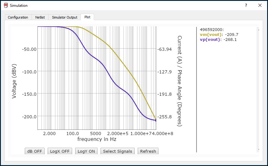
Let’s look at the plot graph a little closer now. Current is on the right, and all of the wavy lines are phase angles. You can see the legend on the right how each line is defined. Vm is magnitude, Vp is phase. But what are these values related to?

Voltage Probes

Move the Simulation dialog aside and look at your schematic. You should see six different blue probes that correspond to data points on your plot. These probes have been set up for each output and were placed using the Voltage Probe  and Phase Probe icons at the top of your interface.

When you place probes, these are the only data points that the SPICE simulator will check for. Probes are ideal if you have a large circuit with a ton of nodes. You obviously don’t want to plot all of them, so you can use probes to simulate specific signals that you care about.

Signal Filtering

Back in our plot, let’s filter out some signals. Press the Select Signals button at the bottom of the Plot tab, and you’ll see on/off toggles on the right. In our example, we want to look at all of the signal magnitudes without the phases. To do this, toggle all of the Vp’s to off and select the Apply Changes button.

You should have the plot graph as shown below after filtering signals:

Now, what are we looking for in this data? This is a filter circuit, so we need to look for the cutoff frequencies. By moving your cursor from left to right, we can see the first cutoff frequency point is at 1.59KHz as expected. Walking down the lines, the next intersection point is at 159KHz, right again. Our final cutoff point is at 15.9KHz, which looks right.

Simulation Round 2

This is some interesting data. Let’s see how tweaking a capacitor value can increase the cutoff frequency. To do this, we’ll select the Netlist tab in the Simulation dialog and change our C3 capacitor from 10p to 1p as shown below. Once changed, press the Simulate button to rerun the simulation.

nce the Plot tab displays, we’ll press the Select signals button and turn off all the signals. We only want to look at the magnitude and phase of the output, so we’ll turn off the following:

• I(v_v1)
• vm(vcap1)
• vp(vcap2)
• vm(vcap2)
• vp(vcap2)

As expected, by changing the frequency and capacitor rating manually we saw that the signal cutoff frequency was a lot higher.

That finishes up our AC sweep example. Let’s summarize some of the features that we learned about today:

• Multipliers. When setting start/end values for DC and AC sweep you can combine units, multipliers, and scientific notation to express values. For examples, 10,000 MHz can be expressed as 1.000e+10.
• Plot Filtering. The plot tab has several handy filtering options. dB OFF will turn off decibel conversion for your signals. Select Signals will allow you to filter which signals you want to be displayed on your plot graph.
• Probes. When placing probes on a schematic, the SPICE simulator will only analyze probed signals, not named nodes. Probes come in handy when you have a ton of named nodes but only want to analyze specific signals.

Sweeping It Up

DC sweep and AC sweep are two powerful simulation methods to add to your SPICE workflow. With DC sweep, you get an accurate representation of how the circuit performs as one of the independent sources is varied. With AC sweep, you can calculate the small-signal response of a circuit. In future blogs, we’ll be looking at our final simulation method, transient point analysis. We’ll also cover how to map SPICE models to existing symbols, and how to make an old schematic SPICE compatible. Be on the lookout for future updates in our SPICE Simulation Series!

Have you been following along? Try the new SPICE simulation for free! Download Autodesk EAGLE 8.4 now.