In finite element (FE) analysis the detail in which a geometry is discretized into nodes and elements determines the system resources and computational time required to calculate the solution. A balance must always be struck between capturing all the complexity of a component and producing simulation results in a useful timeframe. The number of elements required for a static-uniform mesh, scale roughly cubically with the finest feature to be represented. An adaptive mesher, such as the one included in Netfabb Simulation, eliminates this scaling factor by using fine elements only where necessary and updating the mesh with each time step. This allows simulations to be completed with significantly reduced node and element counts, minimizing the computational time.
Static-uniform Finite Element Meshing
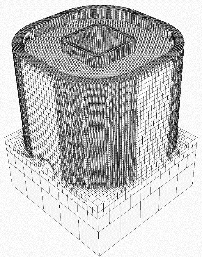
Standard voxel-based FE meshes specify a single uniform element size, which is used to represent the entirety of the geometry. Throughout the transient analysis the mesh remains static. This type of static-uniform mesh is shown below:

Figure 1. Static-uniform mesh with ~1.6 Million nodes & 1.5 Million elements.
Automatically Adaptive Finite Element Meshing
Adaptive meshes reduce the number of nodes in an FE mesh required to complete in simulation by combining sets of 8 small contacting elements into 1 larger element. The nodal reduction occurs over both space and time:
- Adaptivity in space – the mesh density is reduced over a geometry, keeping fine elements at geometric regions which require smaller elements to represent them, and using larger elements to represent bulkier sections
- Adaptivity in time – each time step the mesh is updated to combine elements where possible, so that at every simulated time step, the coarsest feasible FE mesh is used.
Below, is an image of a mesh for the same part, allowing for 1 level of adaptivity is shown:

Figure 2. Mesh using 1 level of adaptivity.
This reduces the nodal count to 378 658 and the number of elements to 267 173.
Here is the mesh, allowing for 5 levels of adaptivity:

Figure 3. Mesh using 5 levels of adaptivity
This further mesh density reduction has just 277 936 nodes and 150 451 elements.
Simulation Results
Part-scale thermo-mechanical simulations are run for each of the 3 example mesh cases using the following settings:
- PRM File: DMG Mori Lasertec30 Ti-6Al-4V 50 Micron
- Build Plate Material: Ti-6Al-4V
- Build Plate Thickness: 15 mm
- Operating Conditions: Estimated heat loss
- Layers Per Element: 5
- Adaptivity Levels:
- 0 (Static-Uniform Mesh)
- 1 (Some adaptivity)
- 5 (Large adaptivity)
Contour plots of the X-Displacement at the end of each simulation for each Mesh Adaptivity option are displayed below:

Figure 4. X-Displacement using a Static-uniform mesh

Figure 5. X-Displacement using 1 level of Adaptivity

Figure 6. X-Displacement using 5 levels of Adaptivity
The results for these three cases are practically identical when compared. This shows that Mesh Adaptivity can be utilized and still maintain simulation accuracy.
Run Time Comparison
The run times for all the meshes above, Static-Uniform, 1 level of Adaptivity, and 5 levels of Adaptivity, are shown in the following table
| Mesh Method | Run time (min) | % Run time reduction over static-uniform |
| Static-uniform | 6368 | Baseline |
| 1 Adaptivity Level | 115 | 98.2% |
| 5 Adaptivity Levels | 23 | 99.6% |
This illustrates the usefulness of Mesh Adaptivity, where using just 1 level of Adaptivity yields simulation time that is just 1.8% of the time required to solved with the Static-uniform mesh. Using 5 levels of adaptivity achieves further time savings, simulating the model in 0.4% of the time required by the Static-Uniform mesh.
Conclusion
It has been shown that Mesh Adaptivity can be used to significantly reduce simulation times while also preserving model accuracy.