& Construction

Integrated BIM tools, including Revit, AutoCAD, and Civil 3D
& Manufacturing

Professional CAD/CAM tools built on Inventor and AutoCAD

Integrated BIM tools, including Revit, AutoCAD, and Civil 3D

Professional CAD/CAM tools built on Inventor and AutoCAD
Run simulations with and without an initial conditions object, and analyze and compare the generated results.
Type:
Tutorial
Length:
8 min.
Tutorial resources
These downloadable resources will be used to complete this tutorial:
Transcript
00:04
When your 1D-2D river model is complete, it can be used for simulations.
00:09
In this tutorial, you create two sets of runs, with and without an initial conditions object,
00:17
and analyze and compare the generated results.
00:21
For more complex 1D-2D models it may be too complicated or onerous to use the initial condition objects.
00:29
In those situations, an initial state file simulation should be used which generates the correct starting conditions for the simulation.
00:39
To begin, open the transportable database .icmt file for this tutorial, copy all of the content to the database.
00:50
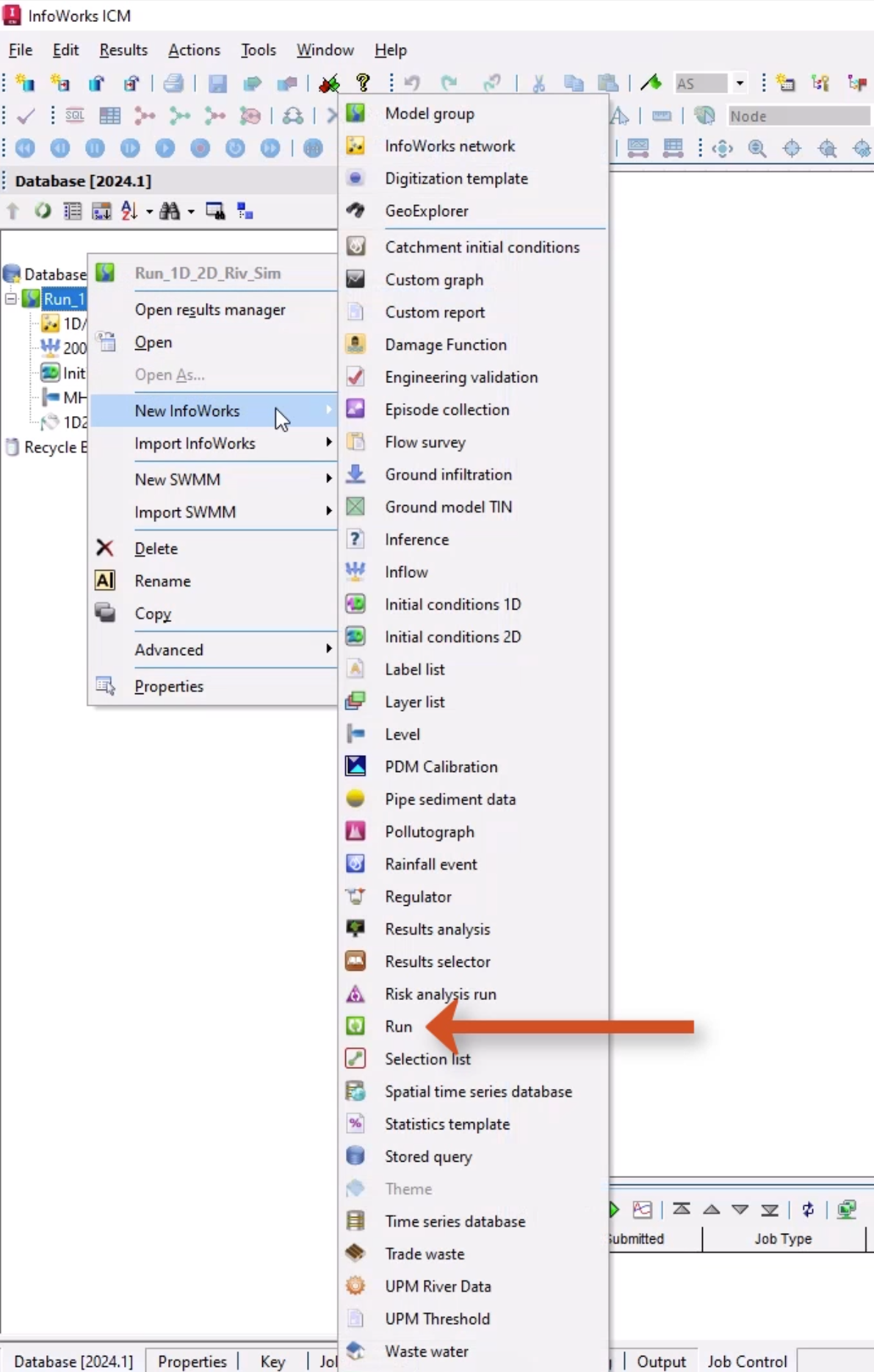
In the Database, right-click the Model Group and select New InfoWorks > Run.
00:58
In the Run window, add a Run title of “1D-2D River Model – No IC”.
01:07
From the Database, drag 1D/2D River Model into the Run window and drop it into the InfoWorks network section.
01:19
Set the following time-related parameters:
01:22
Timestep(s): Set to a more appropriate value of 5
01:27
Results timestep multiplier: 60
01:31
Duration: Set the drop-down to Hours and the amount to 18
01:37
From the Database, drag 200 Year Inflows into the Run window, and then drop it into the Inflow section.
01:46
Drag MHWS 32.255mAD into the Level section.
01:54
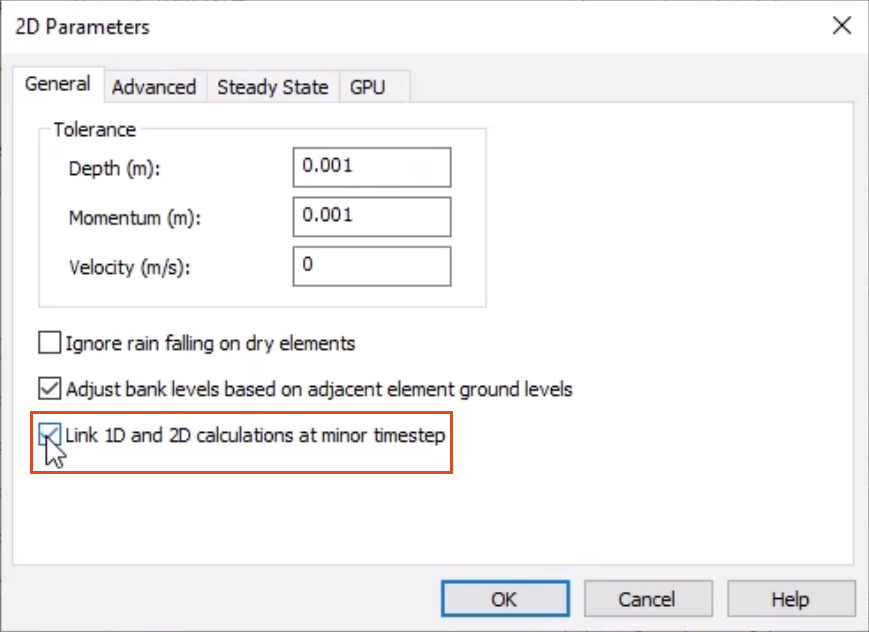
To aid the simulation stability, click 2D parameters,
01:59
and on the General tab, enable Link 1D and 2D calculations at minor timestep.
02:07
Click OK.
02:09
Click Run simulations.
02:11
In the Schedule Job(s) popup, click OK.
02:16
From the Window menu, select Job control window
02:21
to display the status of scheduled simulation jobs.
02:24
In the Database, double-click 1D-2D River Model - No IC
02:31
to open the Run window.
02:33
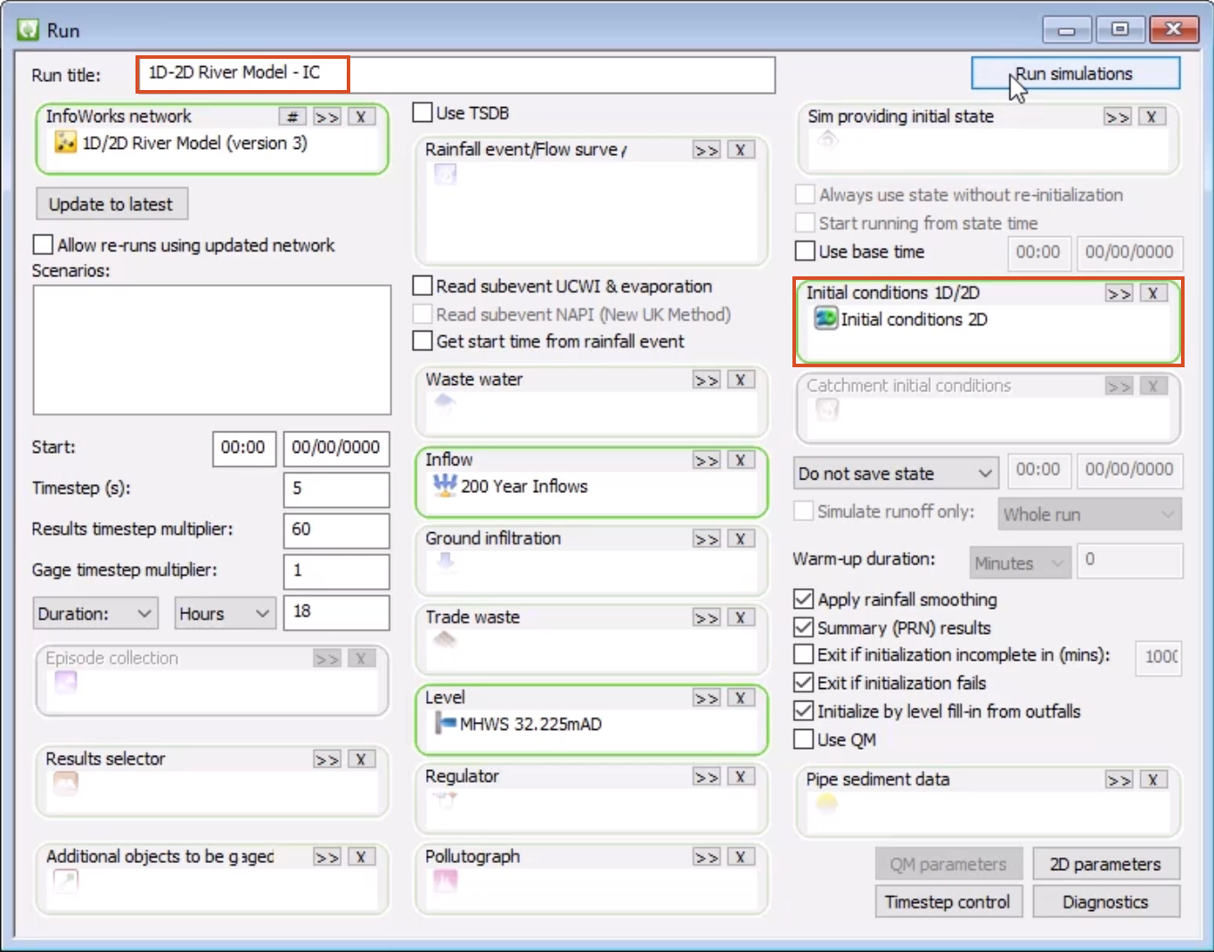
Update the Run title to “1D-2D River Model - IC”
02:39
and from the database, drag the Initial conditions 2D object into the run window to add it.
02:47
Click Run simulations.
02:50
Once the first simulation is complete, you can analyze the results.
02:54
In the Database, double-click the result icon for 1D-2D River Model - No IC to open the simulation on the GeoPlan.
03:05
To help you visualize the results, drag the pre-saved 1D2D River Results theme from the Database onto the results.
03:15
If you need to adjust the theme, right-click the model results and select Properties & themes.
03:23
In the Replay Control toolbar, click Play to start the simulation.
03:29
Notice that the flow starts immediately from the 2D boundary.
03:36
If you query one of the objects close to the boundary, you can see that the 2D mesh was dry when the simulation started.
03:45
The overall impact on this simulation is not significant as it takes around 1 hour to fill this area,
03:54
but it could be for other models, especially if the time to peak was much shorter
03:60
and there was a large volume that needed to be infilled.
04:04
Once the second simulation is complete, open the 1D-2D River Model - IC results.
04:12
Drag the 1D2D River Results theme onto the simulation.
04:18
Unlike the first simulation, within the IC zone, there is water simulated on the surface of the downstream section.
04:28
In the Replay Controls toolbar, select Show Maxima.
04:34
This theme has been set up to show whether the banks are flooding (red) or accepting flow (blue).
04:41
In the GeoPlan Tools toolbar, click Find in GeoPlan and perform a Quick Find for River Reach US.1.
04:52
Once located, Close the Quick Find window.
04:56
Select River Reach US.1 to open the Result Properties window.
05:02
For the Left bank data, Right bank data, and Section data fields, click More (…).
05:11
You can investigate this data to get a better idea of bank and section flow and flooding.
05:17
Use the pick graph tool to select one of the bank lines and graph the bank flow.
05:23
Each section of the river reach bank can be graphed individually.
05:28
It provides a summation of the flow across all the element-bank face connections.
Video transcript
00:04
When your 1D-2D river model is complete, it can be used for simulations.
00:09
In this tutorial, you create two sets of runs, with and without an initial conditions object,
00:17
and analyze and compare the generated results.
00:21
For more complex 1D-2D models it may be too complicated or onerous to use the initial condition objects.
00:29
In those situations, an initial state file simulation should be used which generates the correct starting conditions for the simulation.
00:39
To begin, open the transportable database .icmt file for this tutorial, copy all of the content to the database.
00:50
In the Database, right-click the Model Group and select New InfoWorks > Run.
00:58
In the Run window, add a Run title of “1D-2D River Model – No IC”.
01:07
From the Database, drag 1D/2D River Model into the Run window and drop it into the InfoWorks network section.
01:19
Set the following time-related parameters:
01:22
Timestep(s): Set to a more appropriate value of 5
01:27
Results timestep multiplier: 60
01:31
Duration: Set the drop-down to Hours and the amount to 18
01:37
From the Database, drag 200 Year Inflows into the Run window, and then drop it into the Inflow section.
01:46
Drag MHWS 32.255mAD into the Level section.
01:54
To aid the simulation stability, click 2D parameters,
01:59
and on the General tab, enable Link 1D and 2D calculations at minor timestep.
02:07
Click OK.
02:09
Click Run simulations.
02:11
In the Schedule Job(s) popup, click OK.
02:16
From the Window menu, select Job control window
02:21
to display the status of scheduled simulation jobs.
02:24
In the Database, double-click 1D-2D River Model - No IC
02:31
to open the Run window.
02:33
Update the Run title to “1D-2D River Model - IC”
02:39
and from the database, drag the Initial conditions 2D object into the run window to add it.
02:47
Click Run simulations.
02:50
Once the first simulation is complete, you can analyze the results.
02:54
In the Database, double-click the result icon for 1D-2D River Model - No IC to open the simulation on the GeoPlan.
03:05
To help you visualize the results, drag the pre-saved 1D2D River Results theme from the Database onto the results.
03:15
If you need to adjust the theme, right-click the model results and select Properties & themes.
03:23
In the Replay Control toolbar, click Play to start the simulation.
03:29
Notice that the flow starts immediately from the 2D boundary.
03:36
If you query one of the objects close to the boundary, you can see that the 2D mesh was dry when the simulation started.
03:45
The overall impact on this simulation is not significant as it takes around 1 hour to fill this area,
03:54
but it could be for other models, especially if the time to peak was much shorter
03:60
and there was a large volume that needed to be infilled.
04:04
Once the second simulation is complete, open the 1D-2D River Model - IC results.
04:12
Drag the 1D2D River Results theme onto the simulation.
04:18
Unlike the first simulation, within the IC zone, there is water simulated on the surface of the downstream section.
04:28
In the Replay Controls toolbar, select Show Maxima.
04:34
This theme has been set up to show whether the banks are flooding (red) or accepting flow (blue).
04:41
In the GeoPlan Tools toolbar, click Find in GeoPlan and perform a Quick Find for River Reach US.1.
04:52
Once located, Close the Quick Find window.
04:56
Select River Reach US.1 to open the Result Properties window.
05:02
For the Left bank data, Right bank data, and Section data fields, click More (…).
05:11
You can investigate this data to get a better idea of bank and section flow and flooding.
05:17
Use the pick graph tool to select one of the bank lines and graph the bank flow.
05:23
Each section of the river reach bank can be graphed individually.
05:28
It provides a summation of the flow across all the element-bank face connections.
A complete 1D-2D river model can be used for simulations. This example creates two sets of runs, with and without an initial conditions object, and analyzes and compares the generated results.
Note that for more complex 1D-2D models, it may be too complicated or onerous to use the initial condition objects. In those situations, an initial state file simulation should be used, which generates the correct starting conditions for the simulation.
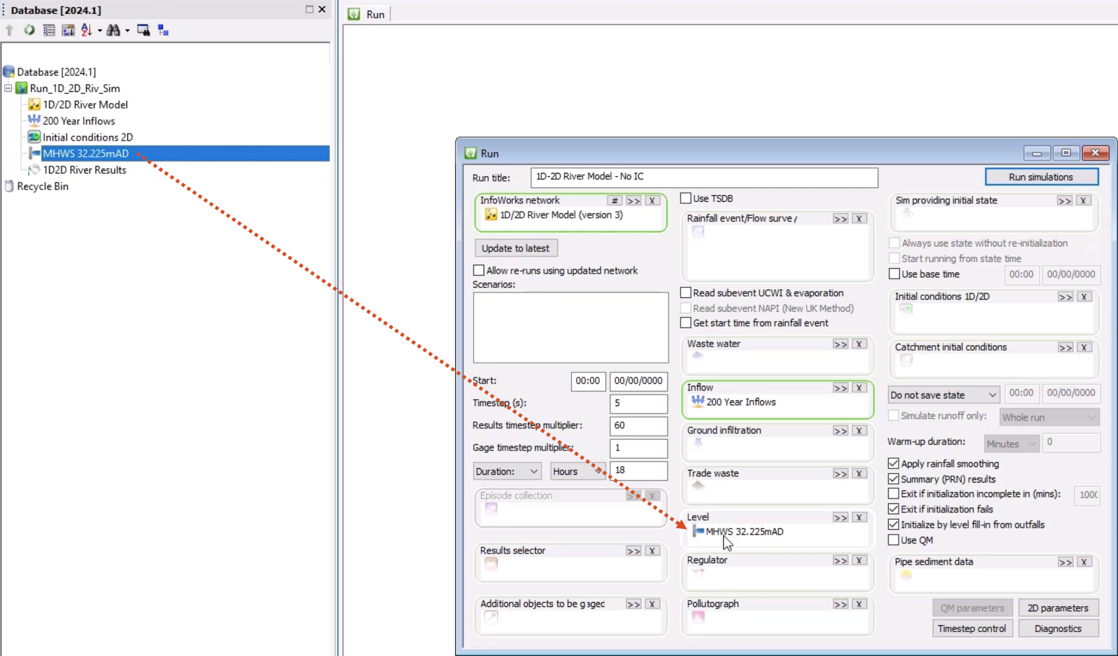
To aid the simulation stability:
Now, set up the second simulation, with the initial conditions object:
Once the first simulation is complete, the results can be analyzed.
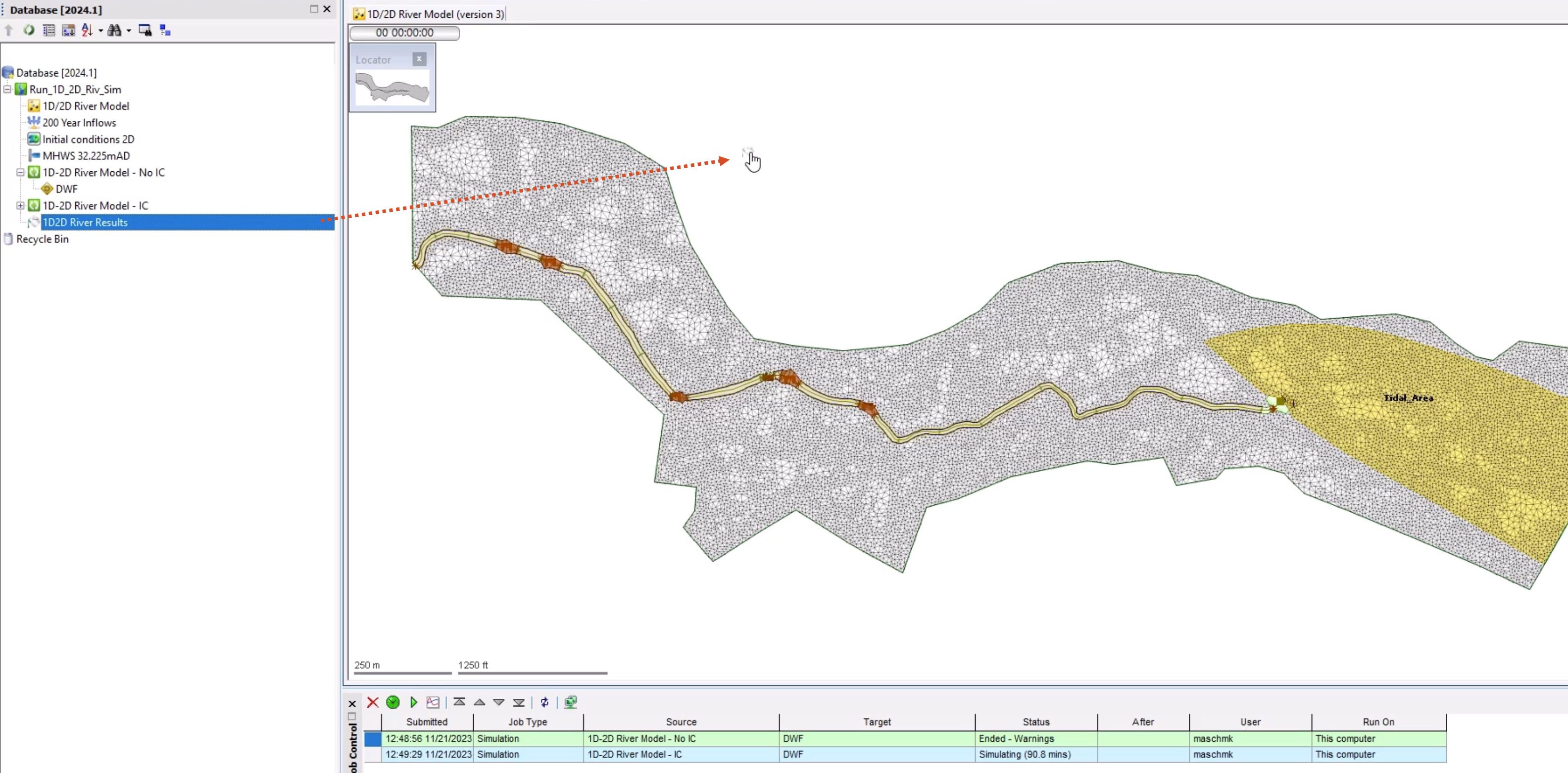
Notice the flow starts immediately from the 2D boundary.
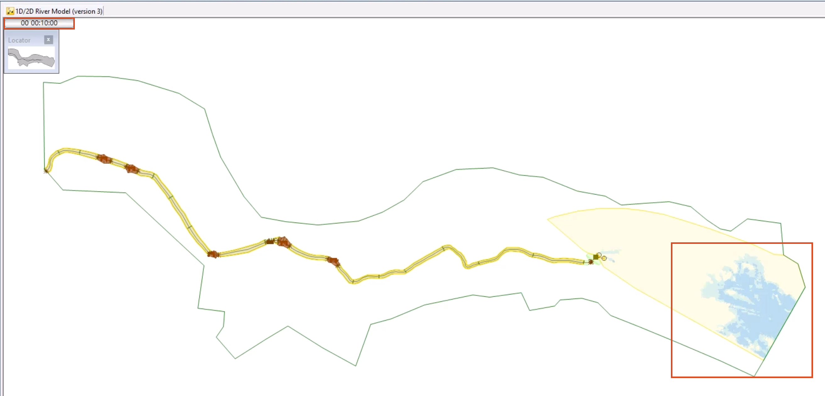
To see that the 2D mesh was dry when the simulation started:
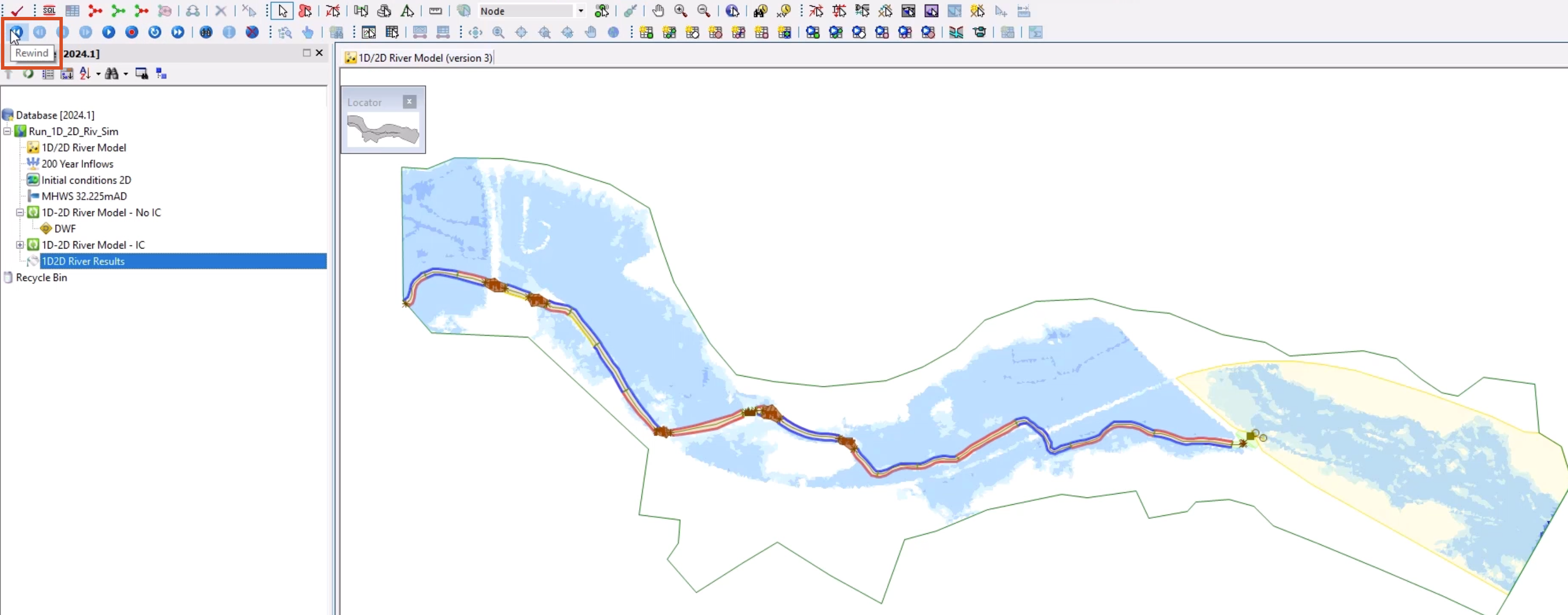
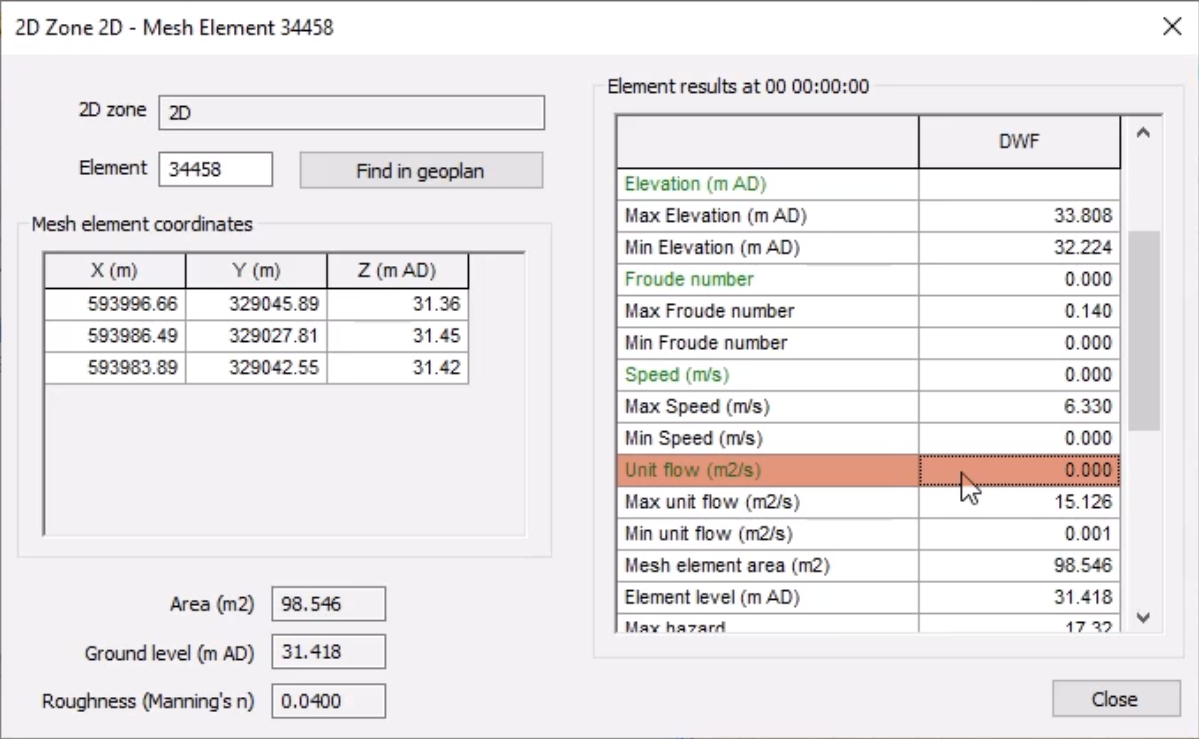
The overall impact on this simulation is not significant, as it takes around 1 hour to fill this area. However, it could be impactful for other models, especially if the time to peak was much shorter, and if there was a large volume that needed to be infilled.
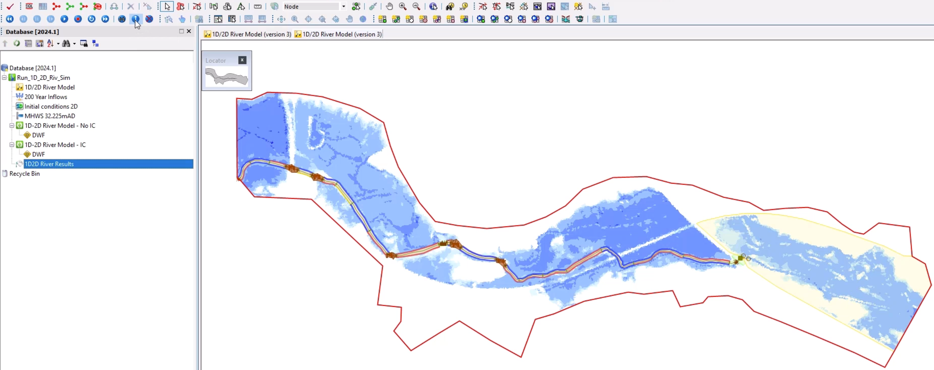
Unlike the first simulation, within the IC zone, there is water simulated on the surface of the downstream section.
This theme has been set up to show whether the banks are flooding (red) or accepting flow (blue).
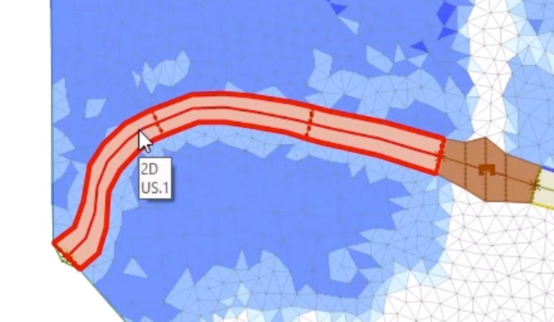
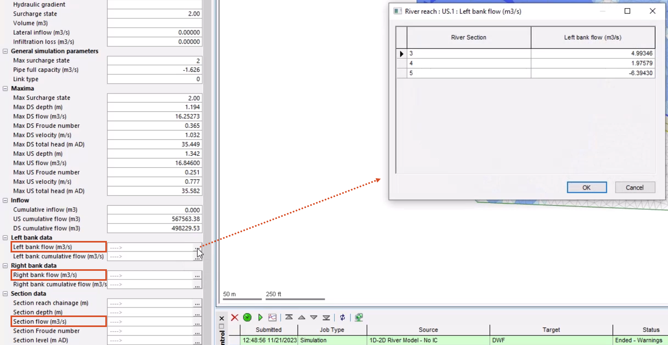
To get a better idea of bank and section flow and flooding, investigate this data:
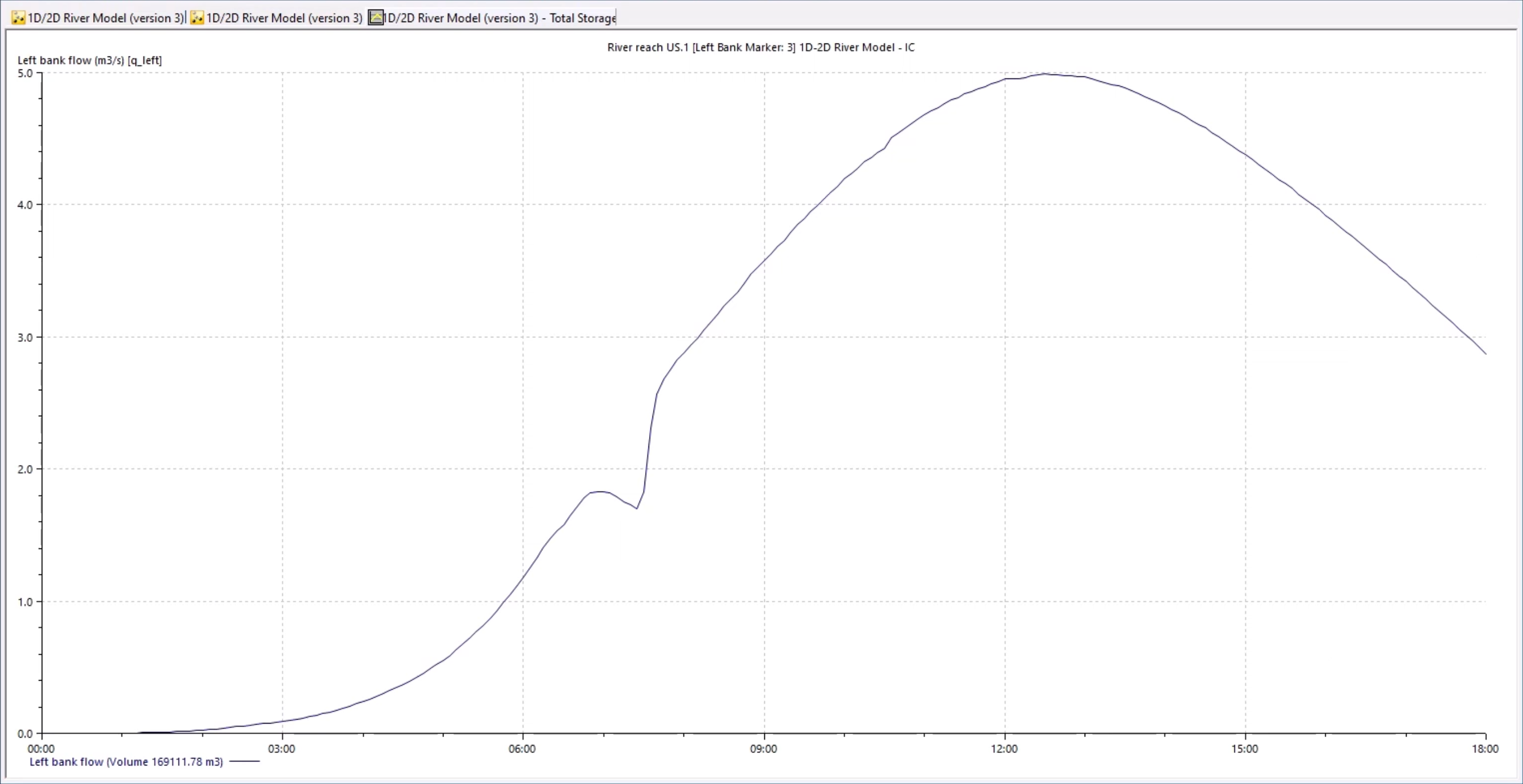
Each section of the river reach bank can be graphed individually. It provides a summation of the flow across all the element-bank face connections.
How to buy
Privacy | Do not sell or share my personal information | Cookie preferences | Report noncompliance | Terms of use | Legal | © 2025 Autodesk Inc. All rights reserved
Sign in for the best experience
Save your progress
Get access to courses
Receive personalized recommendations
May we collect and use your data?
Learn more about the Third Party Services we use and our Privacy Statement.May we collect and use your data to tailor your experience?
Explore the benefits of a customized experience by managing your privacy settings for this site or visit our Privacy Statement to learn more about your options.