Create transients from valve operations

Step-by-step guide

InfoSurge Pro allows hydraulic transients to be created by providing a curve which alters pump and valve operations, as well as junction demand changes. Then, the simulation results from different operational conditions can be compared. In this example, transient events are created from valve operations.

1. Double-click the desired project .aprx file to open ArcGIS Pro.
2. Click the InfoWater Pro tab to open the InfoWater Pro ribbon.
3. In the Project panel, click Initialize.
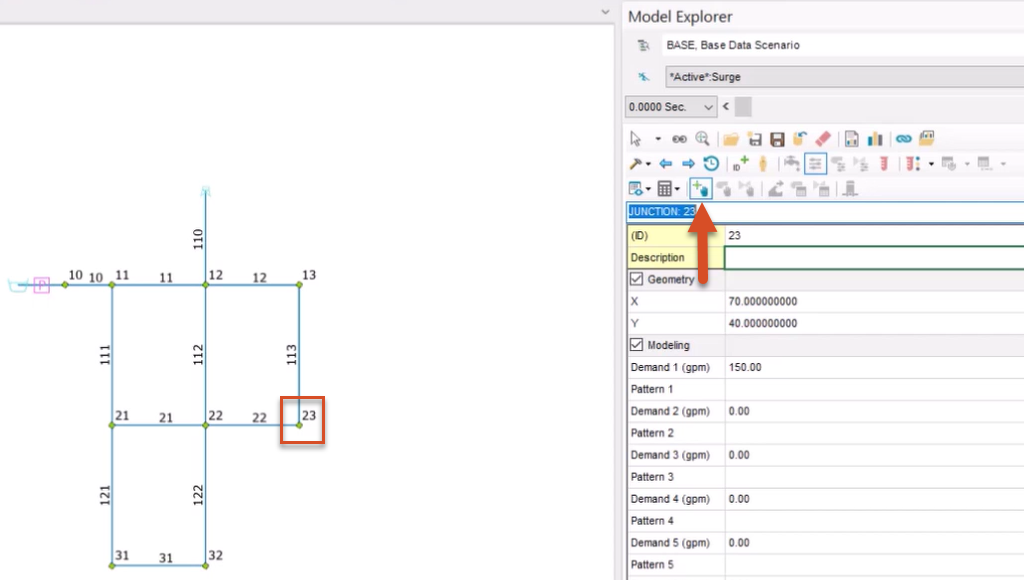
4. From the map, for this example, select Junction 23.
5. From the Model Explorer, select Demand Change to open the Junction Demand Change Data dialog box.

6. Click Purge to remove all existing settings.

Next, create a valve:

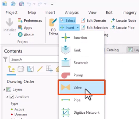
7. From the ribbon, InfoWater Pro tab, Edit panel, expand the Insert drop-down and select Valve.

8. From the map, click the middle of Pipe 111.
9. In the notification about inserting a valve on the pipe, click Yes.
10. In the Valve Identification dialog box, Valve ID field, enter “V1.”
11. Click OK to generate a new valve (V1) and a new pipe (P11).
12. From the ribbon, InfoWater Pro tab, Edit panel, click the Select tool to enable it.
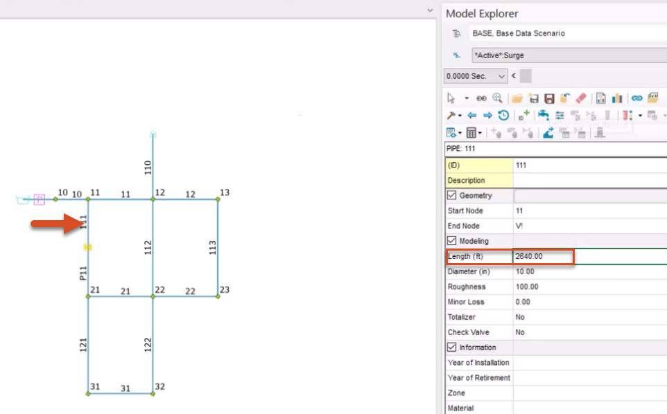
13. Click Pipe 111.
14. From the Model Explorer window, change the Length of the pipe to 2640 feet, or half of the original length.

15. Change the Length of pipe P11 to the same value, 2640.00 feet.
16. Select valve V1.
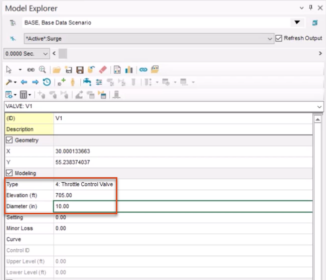
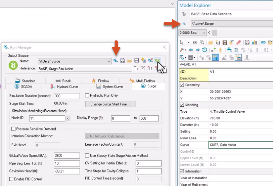
17. From the Model Explorer, change the valve Type to 4: Throttle Control Valve.
18. Set the Elevation to 705 feet.
19. Set the Diameter to 10 inches.

Any change in valve position (% open) will produce a transient. To model this based on valve operation, two curves need to be assigned.

The first is the Active Valve Characteristics curve, which represents the “% stem position” vs. the “minor loss K”. These correspond with the open percentage of the valve (10 = 10% open) and the minor loss coefficient, which accounts for energy lost from flow through the valve.

The second is the Operational Change Data curve, which describes “time” vs. “% stem position”. These curve parameters show the change in how open the valve is (% open) over time.

Together, these two curves account for the valve characteristics and the change in stem position during the transient analysis, respectively.

To calculate the valve characteristics curve:

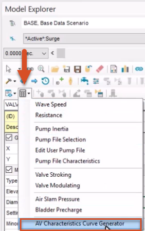
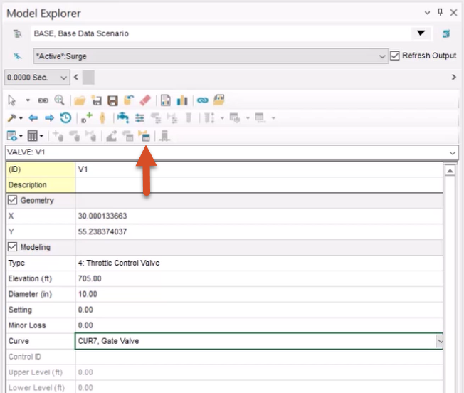
20. From the Model Explorer, click the Auxiliary Calculator button, and in the drop-down, select AV Characteristics Curve Generator.

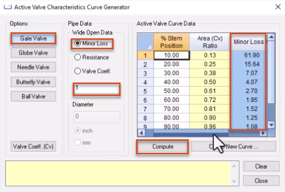
21. In the Active Valve Characteristics Curve Generator dialog box, in the Options group box, click Gate Valve.
22. In the Pipe Data group box, enable the Minor Loss option and enter a value of “1”.
23. Click Compute to calculate the active valve curve.

Note that the Minor Loss K column populates with calculated data.

24. Click Create New Curve to open the New Curve dialog box.
25. In the New ID field, type a name for the new curve. In this example, the name “CUR7, Gate Valve” is entered.
26. Click OK.

Note that in the Active Valve Characteristics Curve Generator dialog box, a message reads: “Curve CUR7 has been inserted into your DB tables.”

27. Click Close.
28. From the map, select valve V1.
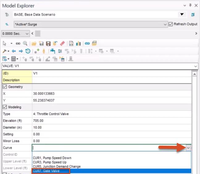
29. From the Model Explorer, in the Curve field drop-down, select CUR7, Gate Valve.

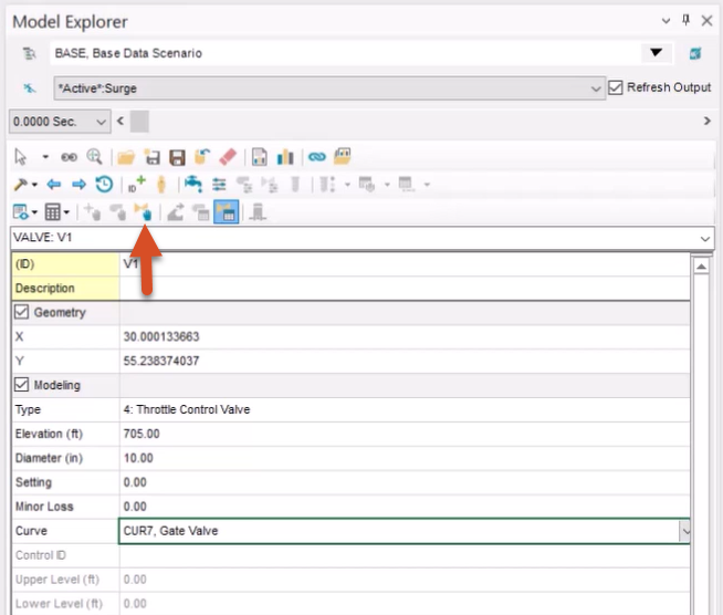
30. Click AV (TCV) Surge Data.

The throttle control valve must be identified as an active valve to use during the surge analysis.

While not used in this example, a bypass line or check valve can be added in this dialog box, if required.

31. In the Active Valve Data dialog box, click Activate to activate the valve.

The Operational Change Data curve for the valve can now be created.

32. From the Model Explorer, click AV (TCV) Operation Change.

This button would not be available if the valve had not been activated.

33. In the dialog box that opens, click Browse (…) to open the Curve dialog box.
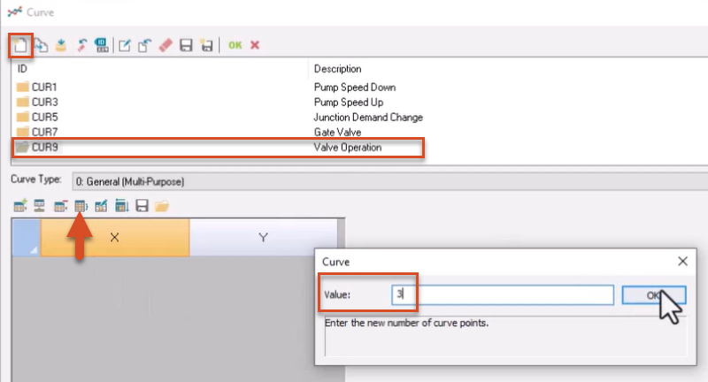
34. Click New to create a new stem change curve.
35. In the New Curve popup, enter a New ID of “CUR9, Valve Operation”.
36. Click OK.
37. Click the Set Rows button.
38. In the Curve popup, assign a Value of “3”.
39. Click OK.

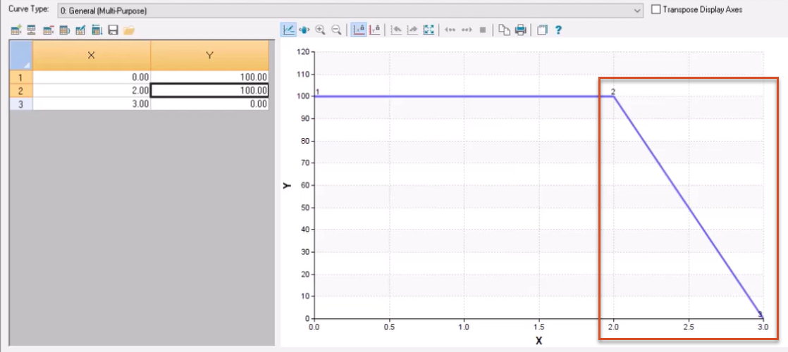
In the table, enter the following values in the X-axis column (time in seconds):

40. In row 1, enter 0.00.
41. In row 2, enter 2.00.
42. In row 3, enter 3.00.

Enter the following values in the Y-axis column (valve % open):

43. In row 1, enter 100.00.
44. In row 2, enter 100.00.
45. In row 3, enter 0.00.

The graph shows that after the first two seconds, the valve turns from fully open to fully closed within the next one second.

46. Click OK to close the Curve dialog box.
47. In the remaining dialog box, click Create.

A surge analysis can now be performed.

48. From the Model Explorer, click Run Manager.
49. In the Run Manager dialog box, click Run to run a surge analysis.

50. Click OK to close the Run Manager.
51. From the ribbon, View panel, click Report Manager.
52. In the Report Manager dialog box, click New.
53. Under Available Output Sources, select *Active*.Surge.
54. From the Graph Report tab, select Surge Node Graph.
55. Click Open.
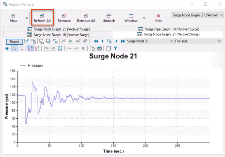
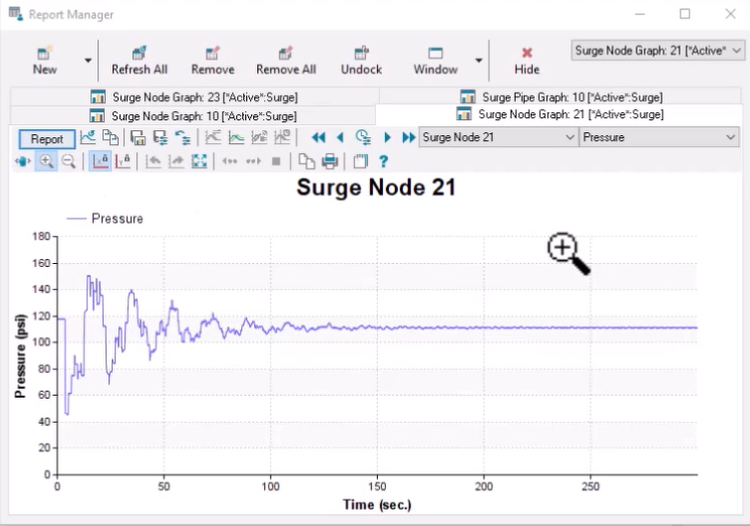
56. From the map, select Junction 21 to view its pressure profile.

Note that closing the valve within one second did create a transient event.

To see how the profile changes with a longer valve operation time:

57. From the Model Explorer, click AV (TCV) Operation Change.
58. Reopen the Curve dialog box.
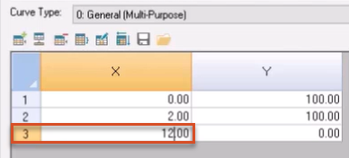
59. In the table, X-column, change the value in the third row to 12.00.

This extends the valve closure time from 1 to 10 seconds.

60. Click OK to close the Curve dialog box.
61. In the Junction Demand Change Data dialog box, click Update.
62. From the Model Explorer, click the Run Manager button.
63. In the Run Manager dialog box, click Run to perform a surge analysis.
64. Click OK to close the Run Manager.
65. From the ribbon, View panel, click Report Manager.
66. From the Report Manager toolbar, click Refresh All to view the new output results.